Team:Minnesota/Modeling
From 2009.igem.org
| (18 intermediate revisions not shown) | |||
| Line 1: | Line 1: | ||
| + | <html> | ||
| + | <style type="text/css"> | ||
| + | table.calendar { margin: 0; padding: 2px; } | ||
| + | table.calendar td { margin: 0; padding: 1px; vertical-align: top; } | ||
| + | table.month .heading td { padding:1px; background-color:#FFFFFF; color:maroon; text-align:center; font-size:120%; font-weight:bold; } | ||
| + | table.month .dow td { color:maroon; text-align:center; font-size:110%; } | ||
| + | table.month td.today { background-color:#AAAAAA; } | ||
| + | table.month td { | ||
| + | border: none; | ||
| + | margin: 0; | ||
| + | padding: 0pt 1.5pt; | ||
| + | font-weight: bold; | ||
| + | font-size: 8pt; | ||
| + | text-align: right; | ||
| + | background-color: #FFFFFF; | ||
| + | } | ||
| + | #bodyContent table.month a { background:none; padding:0 } | ||
| + | .day-active { color:red } | ||
| + | .day-empty { color:black } | ||
| + | |||
| + | </style> | ||
| + | </html> | ||
| + | |||
| + | |||
{|align="center" cellpadding="25" | {|align="center" cellpadding="25" | ||
|[[Image:mnlogo.jpg|300px|center|frame]] | |[[Image:mnlogo.jpg|300px|center|frame]] | ||
|} | |} | ||
| + | {| style="color:gold;background-color:#800000;" cellpadding="3" cellspacing="1" border="1" bordercolor="#fff" width="90%" align="center" | ||
{| style="color:gold;background-color:#800000;" cellpadding="3" cellspacing="1" border="1" bordercolor="#fff" width="90%" align="center" | {| style="color:gold;background-color:#800000;" cellpadding="3" cellspacing="1" border="1" bordercolor="#fff" width="90%" align="center" | ||
!align="center"|[[Team:Minnesota|<font color="gold">Home</font>]] | !align="center"|[[Team:Minnesota|<font color="gold">Home</font>]] | ||
!align="center"|[[Team:Minnesota/Team|<font color="gold">The Team</font>]] | !align="center"|[[Team:Minnesota/Team|<font color="gold">The Team</font>]] | ||
!align="center"|[[Team:Minnesota/Project|<font color="gold">The Project</font>]] | !align="center"|[[Team:Minnesota/Project|<font color="gold">The Project</font>]] | ||
| - | !align="center"|[[Team:Minnesota/ | + | !align="center"|[[Team:Minnesota/Designer|<font color="gold">SynBioSS Designer</font>]] |
!align="center"|[[Team:Minnesota/Modeling|<font color="gold">Modeling</font>]] | !align="center"|[[Team:Minnesota/Modeling|<font color="gold">Modeling</font>]] | ||
| - | !align="center"|[[Team:Minnesota/ | + | !align="center"|[[Team:Minnesota/Notebook|<font color="gold">Experimental</font>]] |
| - | !align="center"|[[Team:Minnesota/ | + | !align="center"|[[Team:Minnesota/Parts Characterization|<font color="gold">Competition Requirements</font>]] |
|} | |} | ||
| Line 17: | Line 42: | ||
[[Image:ModelingLab2.jpg|300px|right|The modelers in their natural environment.]] | [[Image:ModelingLab2.jpg|300px|right|The modelers in their natural environment.]] | ||
| - | + | The primary goal of the modeling group is to create simulations of our experimental results. Our computational output will guide future research and helps us to understand what is happening at the molecular level of our logical AND gate. | |
| + | It is important to be able to observe the fidelity of the AND gate <i>in silico</i> as well as <i>in vivo</i>. Using our in-house software suite, SynBioSS, we will create reaction networks describing the AND gate behavior with different constructs (e.g. TTN, TTL, TNN) and mutations. These reaction networks can then used to create the files necessary for simulation on the supercomputer. Certain kinetic constants in the reaction network can be adjusted to fit the simulation to experimental data. By observing which kinetic constants change with AND-gate construction or mutation we will then be able to understand some of the ways in which the AND-gate functions. | ||
| - | <h2> | + | <h2>Mathematical Modeling</h2> |
| + | <h3>Overview</h3> | ||
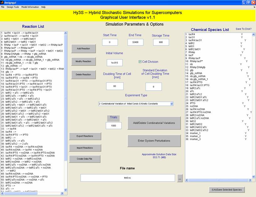
| + | [[Image:designgui.jpeg|300px|left|thumb|The MATLAB GUI displays all the reactions and chemical species in the network and allows the user to manipulate all aspects of the system such as reaction rates in order to better mimic experimental results.]]<p>In order to create a model, we must first use a program that will allow us to enter in the contents of the reactions network. The reaction network is formatted as .nc file, which is a special format called NetCDF that can interact with the group's supercomputer algorithms. The reaction network can be inputted directly into Linux as a text file and then converted into an .nc file. However, this is very tedious and error-prone process. In order to more quickly and accurately create the models, we use one of two programs: SynBioSS or a MATLAB GUI. Each of these programs allows us to graphically see what the model looks like and automatically converts the data describing the system into an .nc file. (See screenshots). <br> | ||
| + | Once the model is created, it is sent to a supercomputer where it is run using hybrid stochastic simulation algorithms created by the Kaznessis group. This algorithm takes the initial conditions of the model along with the reactions and kinetic constants and determines the state of the system over time. A stochastic model is used because the system that is described is very small. Cells are typically on the order of 1E-15 L. Because of this many molecular species exist in small quantities. When there are low numbers of molecules in a system, discrete changes in the number of molecules drastically change the reaction rates. Stochastic models use random number generators to describe the probabilistic nature of stochastic systems. <br> | ||
| + | The results of the models are then retrieved from the supercomputer and analyzed using MATLAB. It is then possible to see if the model ran correctly and if it gave reasonable results. Depending on how the model compares to the experimental data, kinetic constants are changed and then the process of running a model begins again.<br> | ||
| + | The accuracy of the model is determined by the difference in reporter gene expression between the model and the experiments. In order to make reasonable comparison the models must be rescaled, so that the model data matches with the experimental numerically. Basal expression models, which produce the maximum amount of reporter gene, are created for both the experimental and simulation data. This is done by removing the repressor molecules tetR2 and lacR4 from the system. Using this data, it is possible to rescale the model and the experimental data as a percentage of maximum expression. A least squares regression can then be done to determine the difference between the experimental results and the simulation. <br> | ||
| + | Once the simulation is as close to the experimental results as possible a more accurate description of the AND-gate function can be constructed. This can be done by observing how changes in kinetic constants affect GFP expression. Or, using experimental data for mutant constructs, the simulations can be re-fit and the mutation's affect on the reaction network can be quantified. </p> | ||
| - | |||
| - | |||
| - | |||
| - | |||
| - | |||
| - | |||
| - | |||
| - | |||
| - | |||
| - | |||
| - | |||
| - | |||
| - | |||
| - | |||
| - | |||
| - | |||
| - | |||
| - | |||
| - | |||
| - | |||
<h2>Some Basic Modeling</h2> | <h2>Some Basic Modeling</h2> | ||
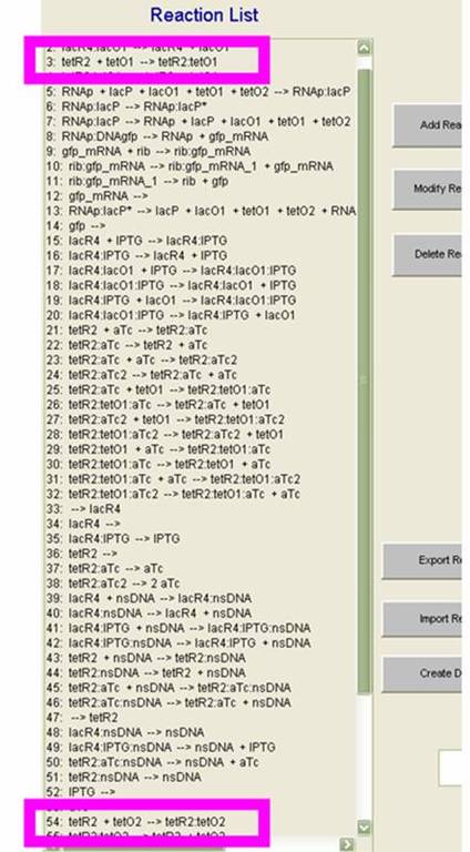
| - | [[Image:reactionlist.jpg| | + | [[Image:reactionlist.jpg|200px|right|The reaction list in the MATLAB GUI with reactions 3 and 54 highlighted.]] |
We are working with four different combinations of <i>lac</i> and<i>tet</i> (L and T, respectively) operators in our promoter design project. These constructs are: T--, TT-, TTL and -T-. Here, we will demonstrate a little basic modeling we have done of the TTL construct using SynBioSS MATLAB and a design GUI. | We are working with four different combinations of <i>lac</i> and<i>tet</i> (L and T, respectively) operators in our promoter design project. These constructs are: T--, TT-, TTL and -T-. Here, we will demonstrate a little basic modeling we have done of the TTL construct using SynBioSS MATLAB and a design GUI. | ||
| - | On the SynBioSS wiki, the TTL model is available for download in a .nc format. Upon opening this with the MATLAB GUI, the list of 65 reactions that constitute the repression and induction of transcription. In this model, there are two <i>tet</i> operators TO1 and TO2 and one <i>lac</i> operator LO1. The reactions included in this list account for the repression and induction of transcription in the absence and presence of aTc and IPTG, respectively. In this simple model, we examined reactions 3 and 54, which involve the <i>tet</i> operators being bound by the repressor. (These reactions are shown in the GUI on the left.) We varied the reactions constants from the original 10<sup>8</sup> as low as 0 and as high as 10<sup>9</sup> to see if the fidelity of the AND gate could depend on the reaction rates for repression. We quantified our results by counting molecules of GFP. This not only gave us a clearer idea of what was happening at the molecular level at this promoter site, but also served as a preparation for matching the experimental results computationally. | + | On the SynBioSS wiki, the TTL model is available for download in a .nc format. Upon opening this with the MATLAB GUI, the list of 65 reactions that constitute the repression and induction of transcription. In this model, there are two <i>tet</i> operators TO1 and TO2 and one <i>lac</i> operator LO1. The reactions included in this list account for the repression and induction of transcription in the absence and presence of aTc and IPTG, respectively. In this simple model, we examined reactions 3 and 54, which involve the <i>tet</i> operators being bound by the repressor. (These reactions are shown in the GUI on the left.) We varied the reactions constants from the original 10<sup>8</sup> as low as 0 and as high as 10<sup>9</sup> to see if the fidelity of the AND gate could depend on the reaction rates for repression. We quantified our results by counting molecules of GFP. This not only gave us a clearer idea of what was happening at the molecular level at this promoter site, but also served as a preparation for matching the experimental results computationally. |
| - | + | <h2>Calendar</h2> | |
| - | + | {| align="center" | |
| - | + | {| style="color:gold;background-color:#800000;" cellpadding="3" cellspacing="1" border="10" bordercolor="#00CCFF" width="62%" align="center" | |
| - | + | !align="center"|{{#calendar: title=Minnesota |year=2009 | month=06}} | |
| - | + | !align="center"|{{#calendar: title=Minnesota |year=2009 | month=07}} | |
| + | !align="center"|{{#calendar: title=Minnesota |year=2009 | month=08}} | ||
| + | !align="center"|{{#calendar: title=Minnesota |year=2009 | month=09}} | ||
| + | |} | ||
| - | + | <h2>Results</h2> | |
| - | + | Place results of models here. | |
| - | + | ||
| - | + | ||
Latest revision as of 19:22, 7 August 2009
| Home | The Team | The Project | SynBioSS Designer | Modeling | Experimental | Competition Requirements |
|---|
Contents |
Our Modeling Goals
The primary goal of the modeling group is to create simulations of our experimental results. Our computational output will guide future research and helps us to understand what is happening at the molecular level of our logical AND gate. It is important to be able to observe the fidelity of the AND gate in silico as well as in vivo. Using our in-house software suite, SynBioSS, we will create reaction networks describing the AND gate behavior with different constructs (e.g. TTN, TTL, TNN) and mutations. These reaction networks can then used to create the files necessary for simulation on the supercomputer. Certain kinetic constants in the reaction network can be adjusted to fit the simulation to experimental data. By observing which kinetic constants change with AND-gate construction or mutation we will then be able to understand some of the ways in which the AND-gate functions.
Mathematical Modeling
Overview
In order to create a model, we must first use a program that will allow us to enter in the contents of the reactions network. The reaction network is formatted as .nc file, which is a special format called NetCDF that can interact with the group's supercomputer algorithms. The reaction network can be inputted directly into Linux as a text file and then converted into an .nc file. However, this is very tedious and error-prone process. In order to more quickly and accurately create the models, we use one of two programs: SynBioSS or a MATLAB GUI. Each of these programs allows us to graphically see what the model looks like and automatically converts the data describing the system into an .nc file. (See screenshots).
Once the model is created, it is sent to a supercomputer where it is run using hybrid stochastic simulation algorithms created by the Kaznessis group. This algorithm takes the initial conditions of the model along with the reactions and kinetic constants and determines the state of the system over time. A stochastic model is used because the system that is described is very small. Cells are typically on the order of 1E-15 L. Because of this many molecular species exist in small quantities. When there are low numbers of molecules in a system, discrete changes in the number of molecules drastically change the reaction rates. Stochastic models use random number generators to describe the probabilistic nature of stochastic systems.
The results of the models are then retrieved from the supercomputer and analyzed using MATLAB. It is then possible to see if the model ran correctly and if it gave reasonable results. Depending on how the model compares to the experimental data, kinetic constants are changed and then the process of running a model begins again.
The accuracy of the model is determined by the difference in reporter gene expression between the model and the experiments. In order to make reasonable comparison the models must be rescaled, so that the model data matches with the experimental numerically. Basal expression models, which produce the maximum amount of reporter gene, are created for both the experimental and simulation data. This is done by removing the repressor molecules tetR2 and lacR4 from the system. Using this data, it is possible to rescale the model and the experimental data as a percentage of maximum expression. A least squares regression can then be done to determine the difference between the experimental results and the simulation.
Some Basic Modeling
We are working with four different combinations of lac andtet (L and T, respectively) operators in our promoter design project. These constructs are: T--, TT-, TTL and -T-. Here, we will demonstrate a little basic modeling we have done of the TTL construct using SynBioSS MATLAB and a design GUI.
On the SynBioSS wiki, the TTL model is available for download in a .nc format. Upon opening this with the MATLAB GUI, the list of 65 reactions that constitute the repression and induction of transcription. In this model, there are two tet operators TO1 and TO2 and one lac operator LO1. The reactions included in this list account for the repression and induction of transcription in the absence and presence of aTc and IPTG, respectively. In this simple model, we examined reactions 3 and 54, which involve the tet operators being bound by the repressor. (These reactions are shown in the GUI on the left.) We varied the reactions constants from the original 108 as low as 0 and as high as 109 to see if the fidelity of the AND gate could depend on the reaction rates for repression. We quantified our results by counting molecules of GFP. This not only gave us a clearer idea of what was happening at the molecular level at this promoter site, but also served as a preparation for matching the experimental results computationally.
Calendar
|
|
|
| ||||||||||||||||||||||||||||||||||||||||||||||||||||||||||||||||||||||||||||||||||||||||||||||||||||||||||||||||||||||||||||||||||||||||||||||||||||||||||||||||||||||||||||||||||||||||||
|---|---|---|---|---|---|---|---|---|---|---|---|---|---|---|---|---|---|---|---|---|---|---|---|---|---|---|---|---|---|---|---|---|---|---|---|---|---|---|---|---|---|---|---|---|---|---|---|---|---|---|---|---|---|---|---|---|---|---|---|---|---|---|---|---|---|---|---|---|---|---|---|---|---|---|---|---|---|---|---|---|---|---|---|---|---|---|---|---|---|---|---|---|---|---|---|---|---|---|---|---|---|---|---|---|---|---|---|---|---|---|---|---|---|---|---|---|---|---|---|---|---|---|---|---|---|---|---|---|---|---|---|---|---|---|---|---|---|---|---|---|---|---|---|---|---|---|---|---|---|---|---|---|---|---|---|---|---|---|---|---|---|---|---|---|---|---|---|---|---|---|---|---|---|---|---|---|---|---|---|---|---|---|---|---|---|---|---|---|---|
Results
Place results of models here.
 "
"


