Team:EPF-Lausanne/Results
From 2009.igem.org
m (→Analysis of the simulation) |
(→Fusion of the LOV domain and the trpR DNA-binding domain) |
||
| Line 23: | Line 23: | ||
//--></script></html> | //--></script></html> | ||
=Fusion of the LOV domain and the trpR DNA-binding domain= | =Fusion of the LOV domain and the trpR DNA-binding domain= | ||
| + | |||
| + | <div style="text-align:justify;"> | ||
The first step in our computational study of the LOV domain was to fuse the 2 domains of interest in VMD. We were then able to visualize the different proteins tried by Sosnick. | The first step in our computational study of the LOV domain was to fuse the 2 domains of interest in VMD. We were then able to visualize the different proteins tried by Sosnick. | ||
The working protein, that we call LovTAP is the result of the fusion at PHE22 of trpR and can be seen on the next video. The general LOV domain is in yellow. Please note the chromophore called Flavin (FMN) in red in the center of LOV2. The trpR dna binding domain is in orange and DNA in gray. | The working protein, that we call LovTAP is the result of the fusion at PHE22 of trpR and can be seen on the next video. The general LOV domain is in yellow. Please note the chromophore called Flavin (FMN) in red in the center of LOV2. The trpR dna binding domain is in orange and DNA in gray. | ||
| Line 63: | Line 65: | ||
* @ALA12: same remarks as for the previous. Furthermore, it is clear that LOV is in interaction with bound DNA. | * @ALA12: same remarks as for the previous. Furthermore, it is clear that LOV is in interaction with bound DNA. | ||
<br><center><object width="425" height="344"><param name="movie" value="http://www.youtube.com/v/FQ-xXnKAYEE&hl=fr&fs=1&"></param><param name="allowFullScreen" value="true"></param><param name="allowscriptaccess" value="always"></param><embed src="http://www.youtube.com/v/FQ-xXnKAYEE&hl=fr&fs=1&" type="application/x-shockwave-flash" allowscriptaccess="always" allowfullscreen="true" width="425" height="344"></embed></object></center></br> | <br><center><object width="425" height="344"><param name="movie" value="http://www.youtube.com/v/FQ-xXnKAYEE&hl=fr&fs=1&"></param><param name="allowFullScreen" value="true"></param><param name="allowscriptaccess" value="always"></param><embed src="http://www.youtube.com/v/FQ-xXnKAYEE&hl=fr&fs=1&" type="application/x-shockwave-flash" allowscriptaccess="always" allowfullscreen="true" width="425" height="344"></embed></object></center></br> | ||
| + | </div> | ||
</div> | </div> | ||
</html> | </html> | ||
| + | |||
=Equilibration of dark state= | =Equilibration of dark state= | ||
We run an equilibration of 80ns on the dark state (2v0u). | We run an equilibration of 80ns on the dark state (2v0u). | ||
Revision as of 13:22, 18 October 2009
Contents |
Fusion of the LOV domain and the trpR DNA-binding domain
The first step in our computational study of the LOV domain was to fuse the 2 domains of interest in VMD. We were then able to visualize the different proteins tried by Sosnick. The working protein, that we call LovTAP is the result of the fusion at PHE22 of trpR and can be seen on the next video. The general LOV domain is in yellow. Please note the chromophore called Flavin (FMN) in red in the center of LOV2. The trpR dna binding domain is in orange and DNA in gray.
Click here to see an example of code used in VMD for the fusion
We also modelized the other fusion tried by Sosnick.
- @MET11
- @ALA12
- @GLU13
- ...
- @PHE22
- ...
- @LEU25
Equilibration of dark state
We run an equilibration of 80ns on the dark state (2v0u).
Here is a movie over the trajectory file.
Validation of the simulation
Here we look at the output to check input parameters.
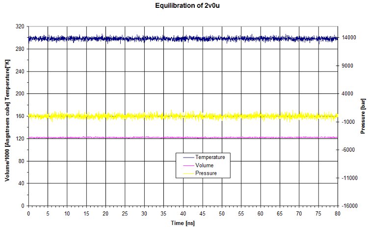
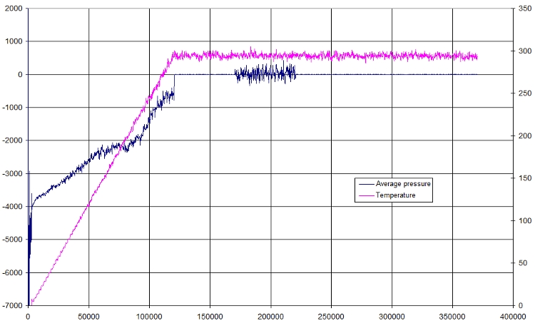
The raw data for the equilibration match what we set for the NPT. Pressure and temperature are kept constant using namd dynamic. The volume is quite constant as well.
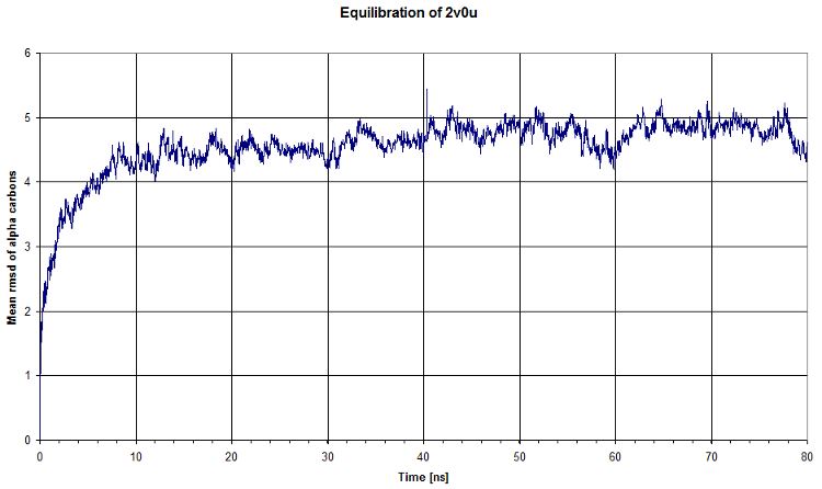
Then we computed the evolution of the rmsd compared to the first timestep of equilibration. We see that there is a plateau after ~40ns, which means that our system's energy is reaching a minimum. That's clearly what we expected.
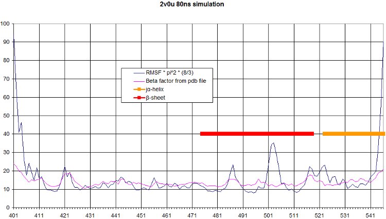
The comparison of the RMSF over the simulation to the beta factor measured during crystallography is a nice validation of our simulation. We get quite similar curves, with some differences at one end of the protein. We see in the movie that this part moves a lot.
Analysis of the simulation
We have organized our analysis on 2 main ideas:
- Find a structural change in the j-alpha helix based on the simulation using namd.
- Find residues showing different comportment in dark and light state
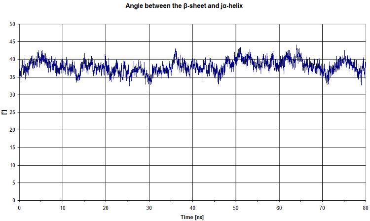
First, we start by looking at the angle between the beta sheet and the j-alpha helix.
Click here to see the code used in VMD to get angle data
We get a quite constant value. It will be more interesting to compare this graph to the light state.
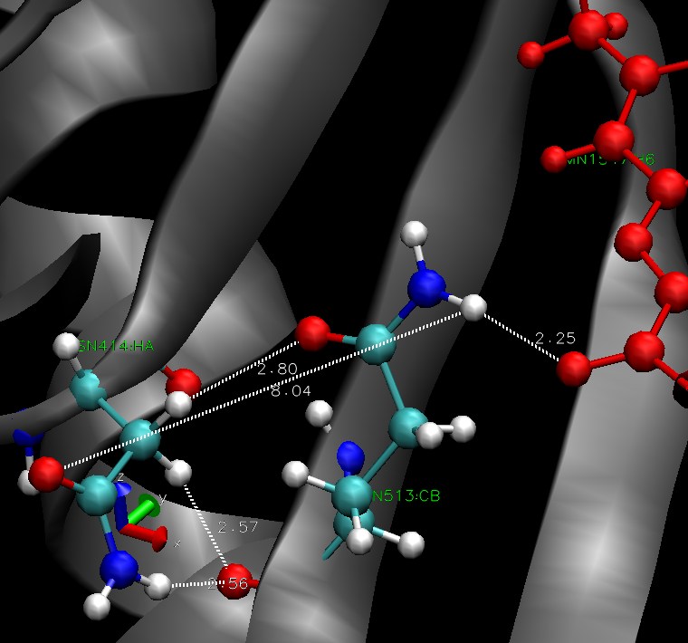
The residues 513 seems to be involved in stabilisation of FMN through hydogen bonds. There is a picture of the situation, residue ASN 414 is on the left, GLN513 in the middle and the FMN is in red. All the hydrogen bonds we investigated over the simulation are pictured.
Equilibration of light state
After having modified some parameters in the parameter files, here is the movie concerning the light state of the protein with the FMN: Light State
Light state
Analysis
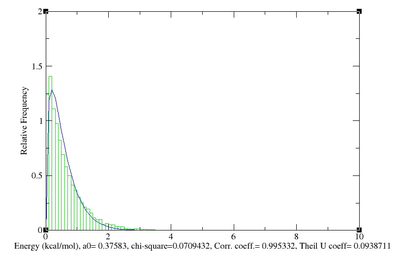
- Maxwell-Boltzmann Energy Distribution
We obtain the following histogramm!
- Temperature
Using EXCEL, we obtain the following graph, which represents the evolution of the temperature in function of time:
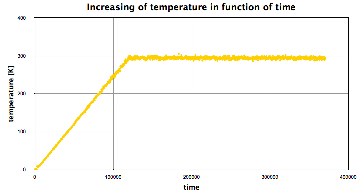
The first part corresponds the the heating, then we let the system reach an equilibrium (NPT state), a NVT portion, and finally a NPT portion again.
- Density
Using EXCEL, we obtain the following graph, which represents the evolution of the density in function of time:
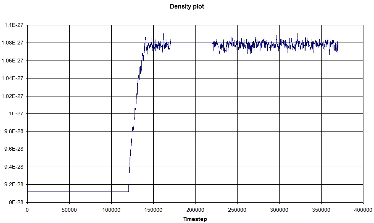
The first part corresponds the the heating, then we let the system reach an equilibrium (NPT state), a NVT portion, and finally a NPT portion again.
- Pressure
Here is a small plot of pressure and temperature in function of time
- RMSD
We obtain the following picture:
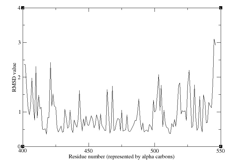
RMSD of residue within 3 angström of the FMN
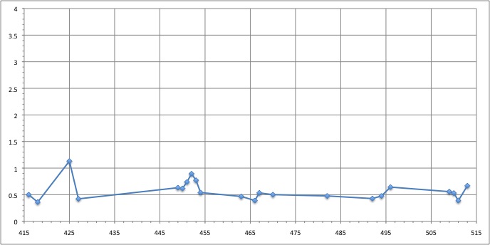
We can see that the residues that move the most are the residue number: 425, 451, 453
RMSD of residue within 6 angström of the FMN
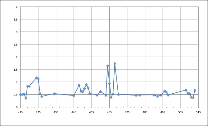
We can see that the residues that move the most are the residue number: 424, 425, 464, 468
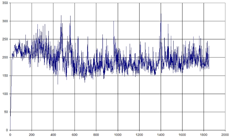
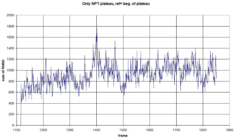
- RMSD of selected atoms compared to initial position along time
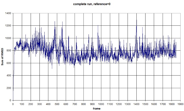
Here is a fast graph of the output of the average RMSD of the atoms in function of time. It seems normal.
Here is what we got with FIRST_FRAME=1115 REFERENCE_FRAME=1115. Average=921.477, standard deviation=202.1708
FIRST_FRAME=0 REFERENCE_FRAME=0. The difference of the sum probably comes from the new selection of atoms from the backbone. We should compute an average value to normalize amplitude. (fluctuation is conserved, anyway) Average=781.3913, standard deviation=118.1393
- Salt bridges
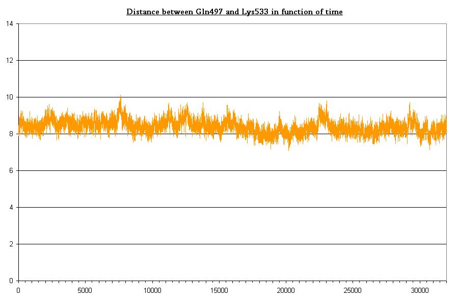
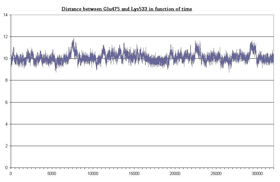
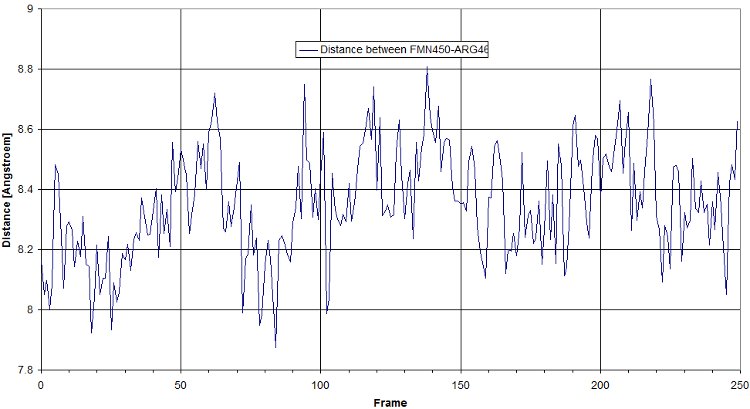
Here is a plot for one of the bridges. We have to look for the max distance for a salt bridge.
- RMSF
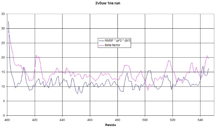
This is a 1 nanosecond NPT run at 300°K. We hope to see a RMSF curve identical to the beta factor. It should only be shifted higher because of the increased temperature. But having a similar tendency would mean our simulation show oscillations similar to what was observed during crystallography. This is really a quite nice validation of our run!
Differential analysis
Some useful distances
- Bond between Gln497 and Lys533 in dark state
- Bond between Gln475 and Lys533 in dark state
 "
"

