Team:Purdue/Modeling
From 2009.igem.org
(→Why Model?) |
|||
| Line 1: | Line 1: | ||
[[Image:Header.png]] | [[Image:Header.png]] | ||
| - | <span style="font-size: | + | <span style="font-size:16px; font-family:georgia; border:2px solid black; padding: 6px; margin: 6px; margin-left:15px;">[[Team:Purdue|<span style="color:green;">Home</span>]]</span> |
| - | <span style="font-size: | + | <span style="font-size:16px; font-family:georgia; border:2px solid black; padding: 6px; margin: 6px;">[[Team:Purdue/Team|<span style="color:green;">The Team</span>]]</span> |
| - | <span style="font-size: | + | <span style="font-size:16px; font-family:georgia; border:2px solid black; padding: 6px; margin: 6px;">[[Team:Purdue/Project|<span style="color:green;">The Project</span>]]</span> |
| - | <span style="font-size: | + | <span style="font-size:16px; font-family:georgia; border:2px solid black; padding: 6px; margin: 6px;">[[Team:Purdue/Parts|<span style="color:green;">Parts Submitted to the Registry</span>]]</span> |
| - | <span style="font-size: | + | <span style="font-size:16px; font-family:georgia; border:2px solid black; padding: 6px; margin: 6px;">[[Team:Purdue/Modeling|Modeling]]</span> |
| - | <span style="font-size: | + | <span style="font-size:16px; font-family:georgia; border:2px solid black; padding: 6px; margin: 6px;">[[Team:Purdue/Notebook|<span style="color:green;">Notebook</span>]]</span> |
| - | <span style="font-size: | + | <span style="font-size:16px; font-family:georgia; border:2px solid black; padding: 6px; margin: 6px;">[[Team:Purdue/Safety|<span style="color:green;">Safety</span>]]</span> |
Latest revision as of 02:08, 22 October 2009
Home The Team The Project Parts Submitted to the Registry Modeling Notebook Safety
NOTE: We highly suggest you read the project description before venturing into this page. The model description assumes that the reader is familiar with the basic processes underlying our system.
Contents |
Why Model?
A mathematical model of a system can be a useful predictive method for a system. In our case, a spatial-temporal model of the kinetics of microglial activation, tat-GFP production, and tat-GFP diffusion can answer such questions as:
- How long will it take until the GFP is detectable?
- What will be intensity of the resulting CD133+ cells?
- Will the diffusion process be limited by diffusion through the membrane or diffusion in the solution?
- How specific will the system be? (i.e., will many cells besides the CD133+ cells be labeled?)
- Will the promoters used be effective, or will a stronger promoter be necessary?
- What happens when the conditions are changed?
Depending on how the model is constructed, all of the above questions and more can be answered without doing a single experiment! (Or by doing very few to determine a few major kinetic parameters).
Assumptions!
Every model contains assumptions. Some assumptions are more valid than others, but in all cases the assumptions simplify the model to make it usable. In our model, we made the following major assumptions as a basic set-up:
- The system lies within a 2-dimensional space
- Our experiments are done in 2-D culture, so any kinetic parameters we measure will apply to the model
- Most processes are simplified into first-order reactions
- Instead of looking at the cell population as a whole, the model generalizes by looking at an "average" cell
- Avoids analyzing the natural cell-to-cell variation
- Uses a single parameter for every cellular process included in the model
- Looking at actual spatial position is unnecessary, as instead we can use the average amount of time to reach a destination
- We will model each distinctly different state of the model as a separate variable, thus eliminating the complexity of looking at the detailed biochemical pathways
Other assumptions concerning each individual step are also made, but these will be detailed later.
The Equations...and what they mean
This mathematical model was constructed using a system of ordinary differential equations. Each equation describes the change in one component over time by summing the effects of other processes on that component (If you don't like math, I promise it's not as complicated as it might look!).
The component names are as follows:
- Mu = "unactivated" microglia
- These microglia are just sitting around, doing what they do best...grow!
- They are "far away" from any CD133+ cells -- i.e., they are not interacting with them
- Mg = microglia "near" glioblastoma
- These microglia are VERY close to the CD133+ glioblastoma cells, but they are not yet touching or interacting
- Mu become Mg when they migrate to the CD133+ cells
- This variable allows the model to describe the rate of movement of the microglial cells toward the CD133+ cells without tracking their spatial path
- Ma = "activated" microglia
- Mg cells become Ma cells when their modified Fc receptors have found and bound the CD133 protein, setting off a signal cascade
- The signal cascade eventually encodes for the production of the tat-GFP construct
- G = CD133+ glioblastoma cells
- TGm = tat-GFP fusion protein in microglia
- This is the concentration of tat-GFP within the microglial cells
- TGe = extracellular tat-GFP
- The concentration of tat-GFP in the extracellular space
- TGg = tat-GFP in CD133+ cells
The units of the microglial and glioblastoma (M and G) cell populations are in cells/um2 (to accomodate the 2-D system). The units of the tat-GFP variables are molecules/cell (for TGm and TGg) and molecules/um2 (for TGe). These units are useful because the system in the model has no definite size. In other words, we do not specify the total number of cells or cell growth area--we just deal in concentrations to be able to model a wider range of situations.
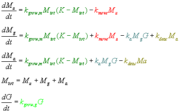
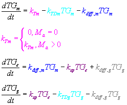
Below are the equations (color-coded for convenience) and, following those, are explanations of each part of the model.
| 
|
As you can see, the majority of the model is based on conservation of mass: if the amount of one component decreases at a certain rate, the amount of another component will similarly increase because the two components are related. Therefore, many parts of the equations are simply repeated from one equation to another. For example, the number of unactivated microglia (Mu) decreases at the same rate that the number of microglia near glioblastoma (Mg) increases because the Mu are becoming the Mg.
- The parts in green describe the growth of the microglia.
- For this, we used the classic logistic model of growth, where the growth rate (kgrow,m) is limited by the size of the area, availability of nutrients, etc.
- The limit of growth is denoted by K (estimated by 95% confluency on a plate).
- The part in lighter green describes the growth of the glioblastoma cells.
- As the cancer cells are immortalized (will not stop growing due to a lack of space or resources), it made sense to use the more basic exponential model of population growth to describe the CD133+ cells
- The parts in red describe the rate of movement of microglia towards the CD133+ cells.
- As the microglia get very close to the CD133+ cells, they "change state" from being "unactivated" to being "near glioblastoma"
- The microglia are assumed to reach the CD133+ cells at some average rate, denoted by kmove.
- The teal text describes the next step of the process, wherein the Fc receptor of the engineered microglia binds the CD133 protein of the glioblastoma
- At this point, the microglia "near glioblastoma" (Mg) become "activated" microglia (Ma).
- The activation of microglia will depend on the concentration of both microglia and glioblastoma (they must actually touch for this to happen), and so this part of the equation is modeled as a 2nd-order reaction
- Activated microglia will begin producing the tat-GFP fusion protein (after some lag time which accounts for the delay caused by the signal cascade as well as the initial transcription of the gene).
- The olive text describes the rate at which the "activated" microglia become "deactivated"
- In other words, this is the rate at which the Fc receptor stops binding to the CD133 protein, stopping the resulting signal cascade and transcription of tat-GFP
- The pink sections detail the rate at which the tat-GFP is produced.
- In this model, the tat-GFP is assumed to be produced at a constant rate in each cell
- The production of tat-GFP is dependent upon the existence of "activated" microglial cells (if there are no actively transcribing microglial cells, there will be no production of tat-GFP)
- The sections in blue describe the diffusion of tat-GFP out of the microglia and into the extracellular space
- The rate of diffusion, according to Fick's law, will be dependent on the concentration of protein (hence the 1st-order reaction)
- The purple step of the process is the uptake of tat-GFP by the CD133+ cells.
- We assume that there is no re-entry of tat-GFP into the microglia once it has diffused out
- The parts in gray describe the possible diffusion of tat-GFP out of the CD133+ glioblastoma cells.
- The parts in cyan describe the degradation of tat-GFP by natural proteases.
- The degradation in the extracellular space is assumed to be zero.
Parameters
We ultimately hope to measure each of the model's parameters ourselves, but for now many of the parameters are estimated based on values found in literature for similar processes. So far, we have been able to estimate growth rates, and we are close to finding the rates of diffusion, uptake, and degradation of tat-GFP.
| Parameter | Description |
|---|---|
| kgrow,g | growth rate of glioblastoma |
| kgrow,m | growth rate of microglia |
| K | limit of microglial growth |
| kmove | rate at which microglia reach glioblastoma |
| ka | rate of microglial activation (rate of binding of Fc receptor to CD133) |
| kdeac | rate of microglial deactivation (rate of un-binding of CD133) |
| kTm | production rate of tat-GFP in microglia |
| kdiff,m | rate of diffusion of tat-GFP out of microglia |
| kdiff,g | rate of diffusion of tat-GFP out of glioblastoma |
| kup | rate of uptake of tat-GFP by glioblastoma |
| kTDg | degradation rate of tat-GFP in glioblastoma |
| kTDm | degradataion rate of tat-GFP in microglia |
Results
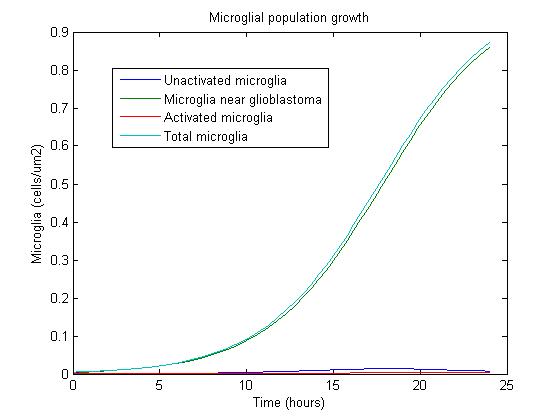
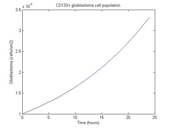
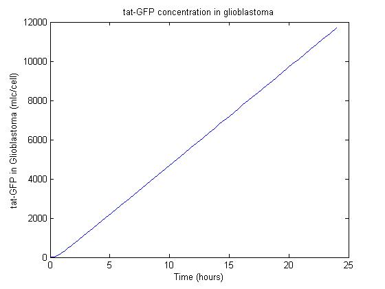
Using some initial parameters, the results of the equations were calculated over a 24-hour period using MATLAB's ODE solver ode23s, which accommodates a constant-mass system.
|
|
|
 "
"
