Team:Bologna/Modeling
From 2009.igem.org
(→Mathematical Model) |
|||
| Line 49: | Line 49: | ||
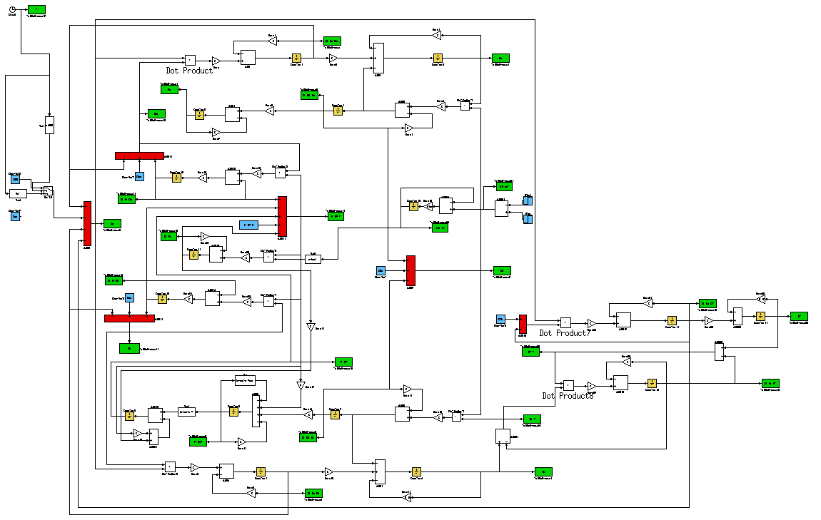
[[Image:ModelSandro.png|center|750px|thumb|Figure 8: Simulink Model]] | [[Image:ModelSandro.png|center|750px|thumb|Figure 8: Simulink Model]] | ||
| - | Results of model simulation are shown in the wet lab parts characterization. | + | Results of model simulation are shown in the wet lab parts [https://2009.igem.org/Team:Bologna/Characterization characterization]. |
Revision as of 02:20, 22 October 2009
| HOME | TEAM | PROJECT | SOFTWARE | MODELING | WET LAB | PARTS | HUMAN PRACTICE | JUDGING CRITERIA |
|---|
A. Einstein
Contents |
Introduction
We developed a mathematical model to simulate the response of the testing circuit (Fig. 1).
Mathematical Model
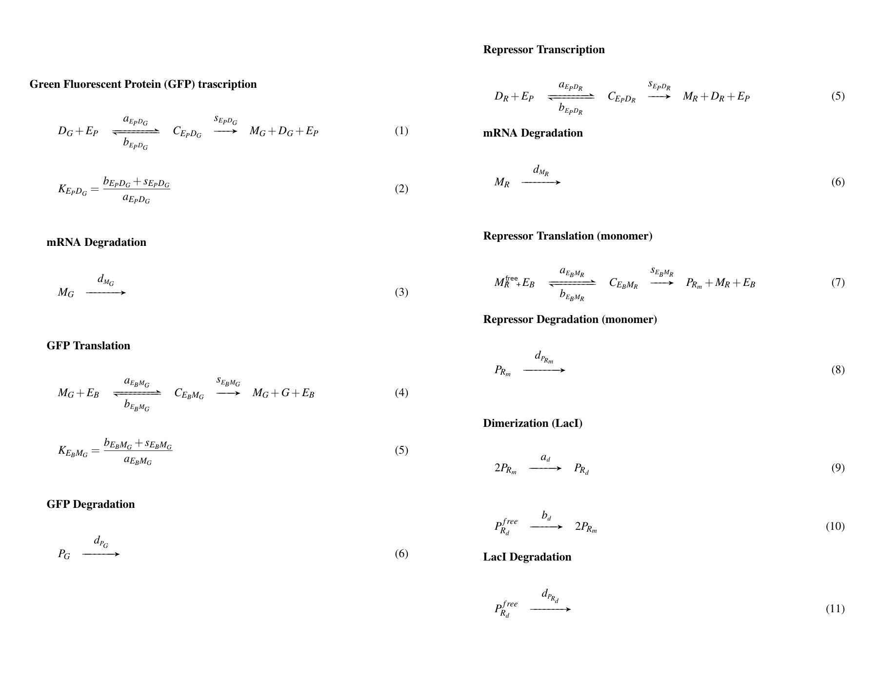
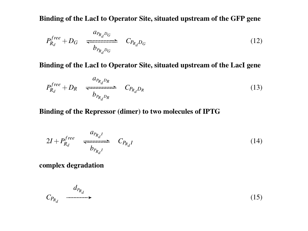
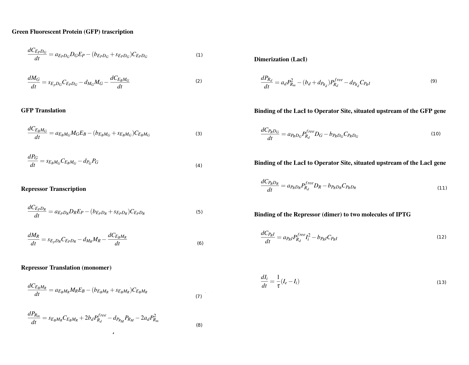
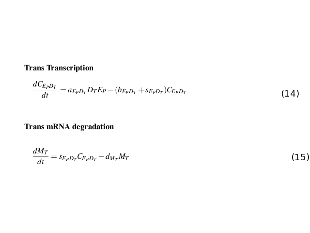
Transcription and translation processes are considered similar to a second order kinetics like an enzymatic reaction: RNA polymerase and ribosome perform enzymes' role, while gene promoter and RBS sequence act as substrates. The binding between enzyme and substrate leads to the formation of a complex, yielding to the final product: mRNA for the polymerase-promoter complex and protein for the ribosome-RBS complex.
Reactions
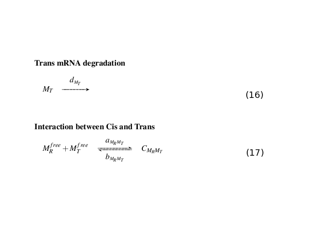
All the biochemical reactions occurring in the testing circuit are listed in Fig. 1, Fig. 2 and Fig. 2
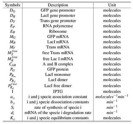
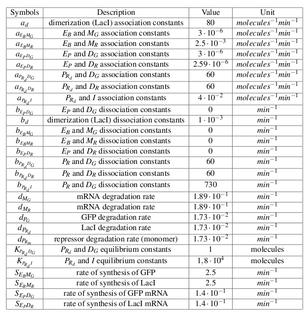
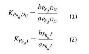
Symbol definitions are listed in Table 1
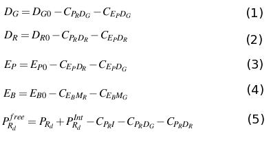
Differential Equations
The differential equations describing the above biochemical reaction are obtained appling the law of mass action.
Simulations
To simulate the model we implemented the equation in Simulink (Figure 3 and Figure 4).
Results of model simulation are shown in the wet lab parts characterization.
 "
"


