Team:McGill/Modeling
From 2009.igem.org

Contents |
Introduction
Many models examining intercellular signaling do not take into account the separation distances of the signaling bodies. We use a partial differential equation (PDE) based model to gain insight into spatially heterogeneous activation-inhibition intercellular signaling.
Two types of signaling molecules exist: activating and inhibiting. Each molecule is synthesized by a unique strain of cells and affects the synthesis rate of the other strain.
This is modeled using the following system of PDEs:
where Ψ1 and Ψ2 represent the concentrations of the activating and inhibiting molecules, respectively, γi the degradation constant, Di the diffusion constant, λi the maximal synthesis rate of molecule i, and δ the Dirac function. fi represents the Hill function describing the dependence on the opposing molecule:
where n, b, and θ are positive. To simplify the analysis, we chose equal parameters between the activating and inhibiting sites (Appendix A).
Numerical Simulation
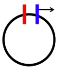
The above system was solved numerically using a forward Euler scheme in time and a centered difference scheme in space. Cyclical boundary conditions were assumed; meaning the spatial dimension formed a ring. This was chosen since simulating an approximate infinite line is computationally costly. However, this also allowed us to investigate two site geometries during one simulation (explained later). The ring was given a physical length of 50 and discretized into 500 intervals. For simplicity, separation distances will be reported in terms of numerical intervals rather than physical distance.
One Oscillator
We first explored the different potential dynamics when the separation distance between an activating and inhibitory site was increased.
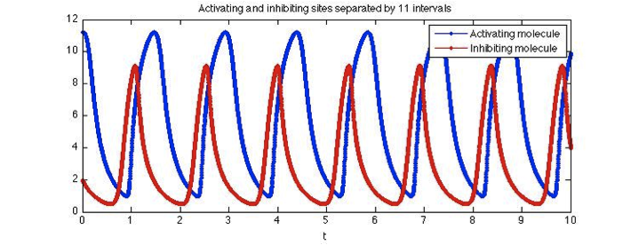
The following is an example of the dynamics observed when the two sites are at a distance where oscillations occur.
Appendix A - Parameters
The standard set of parameters used to observe oscillations were taken directly from Shymko and Glass (1974). γ = 2 D = 2 λ = 54 θ = 1 b = 0 N = 8 Both strains were assumed to have identical parameters in order to simplify the model as well as explicitly observe the dependence of dynamics on separation distance.
 "
"


