 "
"
Team:ULB-Brussels/Project/Mathematical
From 2009.igem.org
(→A first simplified model) |
|||
| Line 54: | Line 54: | ||
We choose a set of values for the different parameters: | We choose a set of values for the different parameters: | ||
| - | [[Image:formule9.png]] | + | [[Image:formule9.png|650px]] |
==== Stationary state ==== | ==== Stationary state ==== | ||
| Line 64: | Line 64: | ||
By solving this system of equations for the previous set of parameters we can find different sets of stationary states. So we have (considering only the states with real values): | By solving this system of equations for the previous set of parameters we can find different sets of stationary states. So we have (considering only the states with real values): | ||
| - | [[Image:formule9c.png]] | + | [[Image:formule9c.png|650px]] |
==== Linear stability analysis ==== | ==== Linear stability analysis ==== | ||
| Line 98: | Line 98: | ||
Given the roots ω<sub>i</sub> of the above equation, we can easily deduce the steady state. From (\ref{a}) it is easy to see that a given state is unstable if any of the ω<sub>i</sub> has a positive real part. In our case we obtain the following expression for [[Image:formule14b.png]]: | Given the roots ω<sub>i</sub> of the above equation, we can easily deduce the steady state. From (\ref{a}) it is easy to see that a given state is unstable if any of the ω<sub>i</sub> has a positive real part. In our case we obtain the following expression for [[Image:formule14b.png]]: | ||
| - | [[Image:formule15.png]] | + | [[Image:formule15.png|650px]] |
Equation (14) is a polynomial of 4<sup>th</sup> order and its first root is of the form: | Equation (14) is a polynomial of 4<sup>th</sup> order and its first root is of the form: | ||
| Line 107: | Line 107: | ||
<ul> | <ul> | ||
| - | <li>set one = [[Image: | + | <li>set one = [[Image:formule16b.png]]</li> |
| - | <li>set two = [[Image: | + | <li>set two = [[Image:formule16c.png]]</li> |
| - | <li>set three = [[Image: | + | <li>set three = [[Image:formule16d.png]]</li> |
</ul> | </ul> | ||
Revision as of 02:02, 22 October 2009

Contents |
Mathematical modeling
Introduction
Synthetic biology is a recent development in biology which aims at producing useful material via biological agents. In this context, a biological system can be seen as a complex network composed of different functional parts (\cite{uri}). Mathematical tools allow one to make prediction on the dynamical behaviour of a given bio-system. We aim at studying the system which has been built in the second section of this report. We already know from our experiment that our system is able to produce glue in the presence of IPTG inductor. We now address the following question: what is the influence of the different parameters on the global dynamics (degradation rate, production rate, level of initial quantity for the C2P22 repressor,...) with and without IPTG. In order to achieve this task, we will consider three different models: the first one shows the basal property we are looking for: a system able to produce glue. The two next models can be seen as two different steps of improvement. The purpose of these models is to improve the experimental control of the glue production. Parameters values result from the literature and previous iGEM team wiki's. We know these remain qualitative and that lab work should be carried out to specify them more precisely.
We start from the global biological system established in the first section (cf. Fig.\ref{fig:without199}(a)). In order to be able to obtain the dynamical equations for the global behaviour of our system, we have to make some assumptions and simplifications. Firstly, we completely neglect the detailed composition of the biobricks. Each of them is considered as a simple block. The next step of our mathematical design is the modeling of the interactions between all the different blocks. The regulation network of our system is modelized using Hill functions for a repressor and an activator. \cite{uri}
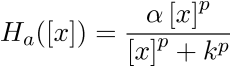
- Hill function for activator :
- Hill function for repressor :
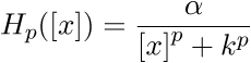


In these expressions, [x] is the concentration of activated genes, p is called the Hill coefficient, k is the activation coefficient and α is the maximum expression level of the promotor.
For each block of the system, we can obtain a dynamical equation by considering its interactions with the other blocks of the system. For each block we can build an equation of the following form: File:Formule3 Where, [x]_i is the concentration of the gene i, R(Ha([x]),Hp([x])) is the regulating function which is a combination of Hill functions. The second term of the right side is the destruction term, where γi is the maximum destruction rate of the gene i.
We must bear in mind, however that the robustness of a given operational regime with respect to external perturbations strongly depends on the value of the Hill coefficients. \cite{arn} In particular, the robustness is expected to increase with the value of the hill coefficient. The cooperativity behaviour is also a function of the Hill coefficient. For these reasons we will consider a situation for which p = 2.
A first simplified model
In this first step, we present a simplified model of our system. We make the following assumptions: we consider that the LuxR+HSL complex is formed quickly at the beginning of the dynamics. This assumption, allows us to modelize the quorum sensing system by considering the complex LuxR+HSL only. The simplified schema is shown on Figure \ref{fig:without199}(b): the effect of the LuxI and LuxR is represented by the autoregulation arrow on the box of the complex LuxR+HSL. We also neglect the effect of the block parE in this first approach.


For the system shown in Figure \ref{fig:without199}(b) we can obtain the following equations (writing here [L] for the LuxR+HSL concentration:
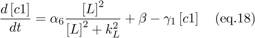
- Equation for the c1 repressor block (designed by c1 in the equation):
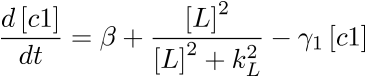
In this equation, the parameter β has the following explicit form:
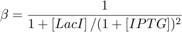
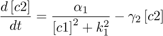
In our case, [LacI] can be considered as a constant, then we have β = β([IPTG]). In this first model we consider only the situation with IPTG inside the system: β ≠ 0. - Equation for the c2 repressor block (designed by c2 in the equation):
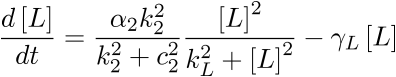
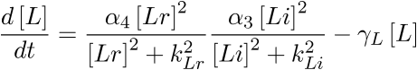
- Equation for LuxR+HSL block (designed by L in the equation):
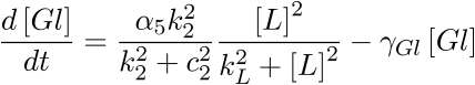
- Equation for the glue production (designed by Gl in the equation, or by hfsGH in the text)


We choose a set of values for the different parameters:
![]()
Stationary state
The first step of our analysis is the study of the stationary point. In order to do that we consider the following algebraic system:

By solving this system of equations for the previous set of parameters we can find different sets of stationary states. So we have (considering only the states with real values):

Linear stability analysis
To check the stability of the stationary states, we perform a linear stability analysis. To this end, we assume that the configuration of the system is perturbed by:
![]()
ω is the growth rate of the perturbation.

is the vector representing the perturbation of each concentration. Linearizing the equations, we can rewrite them in the following form \cite{nico}:
 (11)
(11)
where

and

is the Jacobian matrix. Taking into account the form of the perturbation (\ref{a}), we can write the equation (11) as follows:
![]()
and the eigenvalues ω satisfy the characteristic equation:
![]()
Given the roots ωi of the above equation, we can easily deduce the steady state. From (\ref{a}) it is easy to see that a given state is unstable if any of the ωi has a positive real part. In our case we obtain the following expression for ![]() :
:
![]()
Equation (14) is a polynomial of 4th order and its first root is of the form:
![]()
The others are the roots of a polynomial expression of the third order. We could obtain these roots analytically but their expressions are too complicated to be useful. So, we solve numerically the equation for the previous sets of parameters and we put into the equation (15) the corresponding values for the different sets of stationary states. We have:
- set one =

- set two =

- set three =

Two states are stable and the last one is unstable. The system can stay near its initial configuration, which corresponds to the second set of values or it can also go to another state for which we have glue production (first set). To learn more about the dynamics of this system, we need to study its complete behaviour.
Global dynamics
In order to have an overview of the dynamics of the system we perform a numerical integration of the dynamical equations with the set of previous values for the different parameters. When we solve the system, we see that the system travels from its initial configuration to the nearest stationary stable state which is the second set, corresponding to a state without glue production. We have to stress that we do not find any different situation by varying the set of parameters. We have always a stationary state with no glue production: the system chooses this final configuration. In order to force the system to go to the other state, we add a little basal production term (κ) in the dynamical equation for the complex LuxR+HSL:

noindent In this case, as we can see on the Figure below, the system reaches the first stationary state, for which we have a glue production.
 Dynamical evolution of the concentrations |
 Dynamical evolution of the glue concentration |
Discussion
In this first attempt to obtain a mathematical model of our biological system, we have been able to build a model for which we can obtain stable stationary states with or without glue production. The problem is the following one: the system shows a sensitiveness to the values of the different parameters and the only way to obtain the glue is to introduce a basal production term. The presence of this term is not unrealistic but it is clear that an improvement of this model is needed in order to obtain a dynamical system for which the switch from a state without glue to a state with glue is regulated by the value of β, meaning by the concentration of the inductor in the system (which is the control parameter from the experimental point of view). This is not the case with this simplified model because with κ ≠ 0 we have a glue production independently of the value of β.
Detailed model for the Quorum Sensing system
The aim of this section is to present a more realistic system in order to solve the problem pointed out in the last section. The main difference in this new model is the following one: as we can see on the figure below, we consider a more complete description of the quorum sensing system by taking into account the presence of the LuxR and LuxI blocks. We also consider the effect of the parE block.
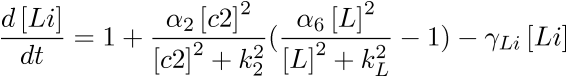
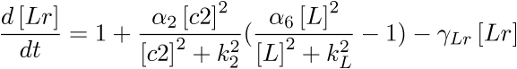
For the system shown on previous figure we have the following equations (writing here [Li] for the LuxI concentration and [Lr] for the LuxR concentration):
- Equation for the c1 repressor block, which is the same as in the previous model:
- Equation for the c2 repressor block, which is the same as in the previous model:

- Equations for the LuxI block and LuxR block: this is the mean improvement in this model.
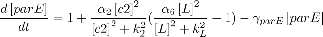
- Equation for parE block, this is a new equation:
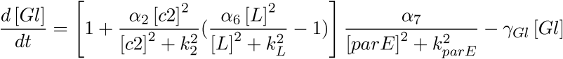
- Equation for the HfsGH block (Gl in the equation), it is almost the same form as before, but there is the effect of the parE block:
- Equation for LuxR+HSL block:
 There is no explicit auto regulation in this model.


In the two next sections of this study we will consider the following set of values for the different parameters which appear in our model:

Considering this set of values, we will study the dynamical behaviour of our system in absence of IPTG and when the inductor is added. We will focus mainly on the influence of the initial value of the [c2] concentration and on the quantity of IPTG which is added in the system. These two concentrations are the main values which can be controlled from an experimental point of view. In the last section of this part, we will discuss the behaviour of the system when some of the intrinsic parameters are modified.
Dynamics of the system without inductor
Steady state
In absence of an inductor (β = 0), the system is expected to stay at rest and not to produce a large amount of glue. We then consider the following initial conditions:
![]()
Due to the complexity of the system we do not expect that it will stay at rest with these initial values but that at least this state will be stable. Indeed, if we try to obtain the steady state by considering the set of algebraic equations obtained by assuming that the time derivatives of all concentrations are set to zero:

It can be seen (for the set of values which has been chosen) that the system will reach a steady state near the initial configuration (It has to be noticed that the glue (hfsGH or Gl in the model) continues to oscillate near zero then it is numerically impossible to obtain a true stationary state for which d[Gl]/dt is strictly zero.) ( [c2] increases to a very high value and the other variables go to almost zero).
Linear stability analysis
As previously explained, we assume that the configuration of the system is perturbed by :
![]()
with

and

The eigenvalues ω satisfy the characteristic equation:
![]()
In this case we obtain the expression:
![]()
This is a polynomial of 7th order and all its roots are of the form:

As we can see, the expression is much more simpler that the one we obtained in the first model. From the linear analysis point of view, the system can reach any stationary state.
 Bifurcation diagram in function of the initial value of [c2] |
 Time evolution of the glue concentration, for values of [c2](t= 0) = 10,20,30,40,50, with β = 0 |
On previous figure (right) we show the time evolution of [hfsGH] for different initial values of [c2], we see that a higher value of [c2] tends toward a diminution of the maximum value of [hfsGH] concentration. As we can see its value is very low, there is just a small increase at the beginning. During the same time the [c2] concentration reaches its steady state. Its concentration is very high; this is mainly due to the fact that the other variables as [L] or [c1] (which can repress [c2]) go to a insignificant value.
Existence of a critical value for [c2]
We have to stress that there is a minimum value for [c2] which has to be found in the system at the beginning. Indeed, as it can be seen on previous figure on the left, when the initial concentration [c2] is too small, the production of glue can start without inductor. The initial concentration [c2] has to be sufficiently high so that the c2 repressor can really represses the other blocks in the system. The critical value for [c2] depends on the parameters of the components of the system so that αi, γi and ki: [c2]c = [c2]c(αi,&gammai,ki).
Dynamics of the system with inductor
 (a):Diagram in function of the amount of inductor for different initial values of [c2] |
 (b): Evolution of the different concentrations for [c1],[c2],[hfsGH] and [L] inside the system with IPTG (model without toggle switch), for initial value of [c2]: 10,20,30,40,50 (quantities have been rescaled) |
When IPTG is added, the system leaves its initial configuration (25) and starts producing glue. Eventually, the system settles down in a steady glue producing state. On Figure (b) we show the dynamical evolution of the system in the presence of IPTG. As we can see the production of the glue begins when the repressor [c2] reaches its final value. During the decrease in [c2], [c1] symmetrically increases. When the production of the glue begins, [c1] rapidly increases to reach its steady value. In this system only a few amount of IPTG is enough to start the process (independently of the initial value of [c2]), as we see on Figure (a). We also have to notice that the concentration of [Li] and [Lr] follows the same temporal evolution as the [L] complex,this is due to the symmetry of the system. The initial value of [c2] concentration does not have any influence on the final amount of produced glue , but the initial value of [c2] has an influence on the rate of the global process: if we increase [c2], the system will take more time to begin the glue production.
In this new model, we see that the glue production can be controled by adding IPTG. But, the system is now too sensitive to the presence of the inductor. In the next section we show how this problem can be solved.