Team:Aberdeen Scotland/internal/stochastic
From 2009.igem.org
(→Stochastic Simulations) |
|||
| Line 9: | Line 9: | ||
1. Choose a time, τ, which is large enough so that all reactions have a possibility of taking place, but small enough so that not too many reactions take place. This is the leap condition from [1]. | 1. Choose a time, τ, which is large enough so that all reactions have a possibility of taking place, but small enough so that not too many reactions take place. This is the leap condition from [1]. | ||
| - | 2. Generate a random number froma Poisson distribution with mean λ=ζ.τ | + | 2. Generate a random number froma Poisson distribution with mean λ=ζ.τ, where τ is the chosen time interval for the stochastic simulation, and ζ represents a term on the right hand side of the ordinary differential equation from the deterministic model.[2] |
| - | + | ||
| - | + | ||
| - | + | ||
3. Multiply each term in the deterministic equations by tau. | 3. Multiply each term in the deterministic equations by tau. | ||
| Line 22: | Line 19: | ||
6. We have now replaced each term in the deterministic equations with an integer distributed around the value of the original term, so we simply add or subtract the integers from the old value of [X_t] to create [X_(t+tau)] | 6. We have now replaced each term in the deterministic equations with an integer distributed around the value of the original term, so we simply add or subtract the integers from the old value of [X_t] to create [X_(t+tau)] | ||
| - | This process can be very fast | + | This process can be computationally very fast depending on the choice of tau. We ran several simulations to determine the dependence of the results on tau and found that the results were robust for tau between ~0.01 seconds and ~1.5 seconds. As expected, the larger tau is, the quicker the simulation runs. We see the comparison between tau = 0.01 seconds, tau = 0.1 seconds and tau =1.5 seconds below. |
| Line 32: | Line 29: | ||
| - | The three simulations with different tau timesteps | + | The three simulations with different tau timesteps yield almost identical results. We not however that the simulation results become non-meaningful for tau larger than 2s (results not shown here). |
== References == | == References == | ||
[1] Gillespie, | [1] Gillespie, | ||
| + | |||
| + | [2] T. Tian, K.Burrage, P. M. Burrage and M. Carletti (2006): Stochastic Delay Differential Equations for Genetic Regulatory Networks, Special Issue of J. Comp and Applied Maths, doi:10.1016/j.cam.2006.02.063 | ||
{{:Team:Aberdeen_Scotland/break}} | {{:Team:Aberdeen_Scotland/break}} | ||
Revision as of 12:59, 14 August 2009
University of Aberdeen - Pico Plumber
Stochastic Simulations
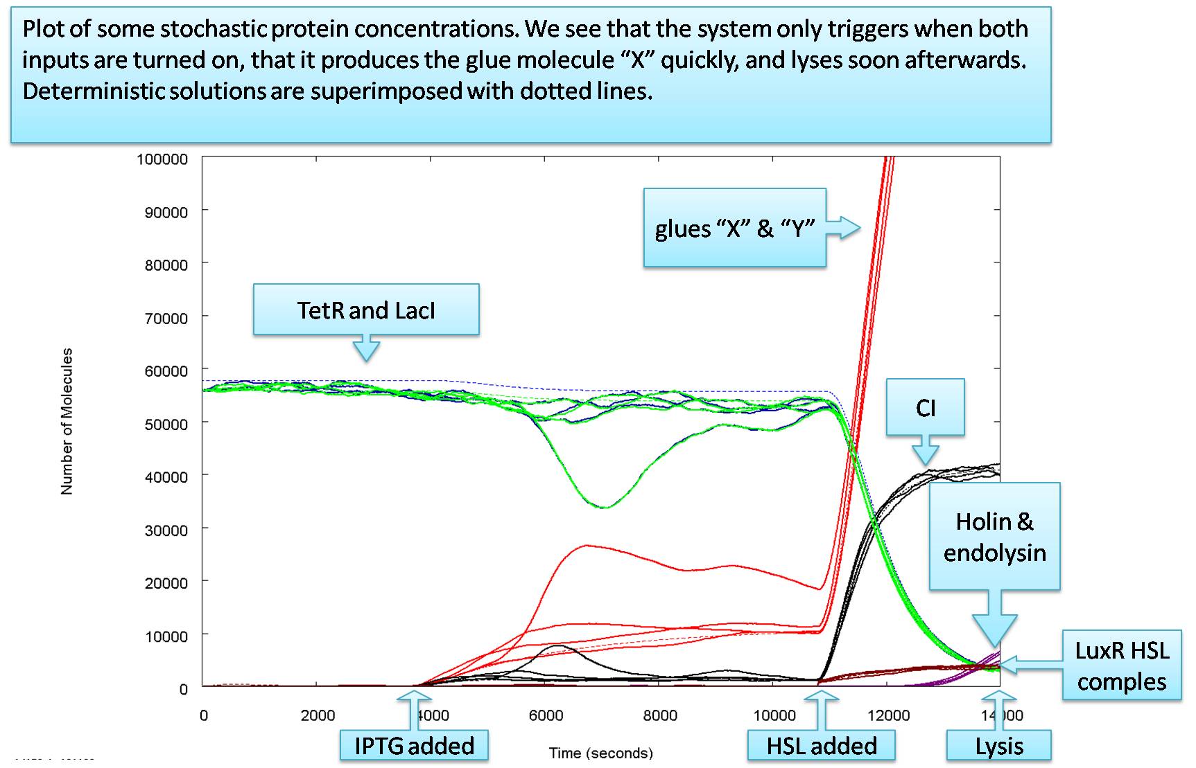
Due to the low levels of proteins involved when the input signal is activated (LacI repression being lifted and the subsequent lifting of the repression of TetR that induces lysis) we decided to perform a stochastic simulation of the model to take into consideration stochastic effects not reproduced by the deterministic model. The method we chose was the “Tau Leap” model - as is it is quite computationally efficient and easy to integrate when a deterministic model has already been established. The method can be implemented by the following simple steps:
1. Choose a time, τ, which is large enough so that all reactions have a possibility of taking place, but small enough so that not too many reactions take place. This is the leap condition from [1].
2. Generate a random number froma Poisson distribution with mean λ=ζ.τ, where τ is the chosen time interval for the stochastic simulation, and ζ represents a term on the right hand side of the ordinary differential equation from the deterministic model.[2]
3. Multiply each term in the deterministic equations by tau.
4. Assign the label λ to the new value of each term.
5. Input the value of λ into the Poisson random number generator
6. We have now replaced each term in the deterministic equations with an integer distributed around the value of the original term, so we simply add or subtract the integers from the old value of [X_t] to create [X_(t+tau)]
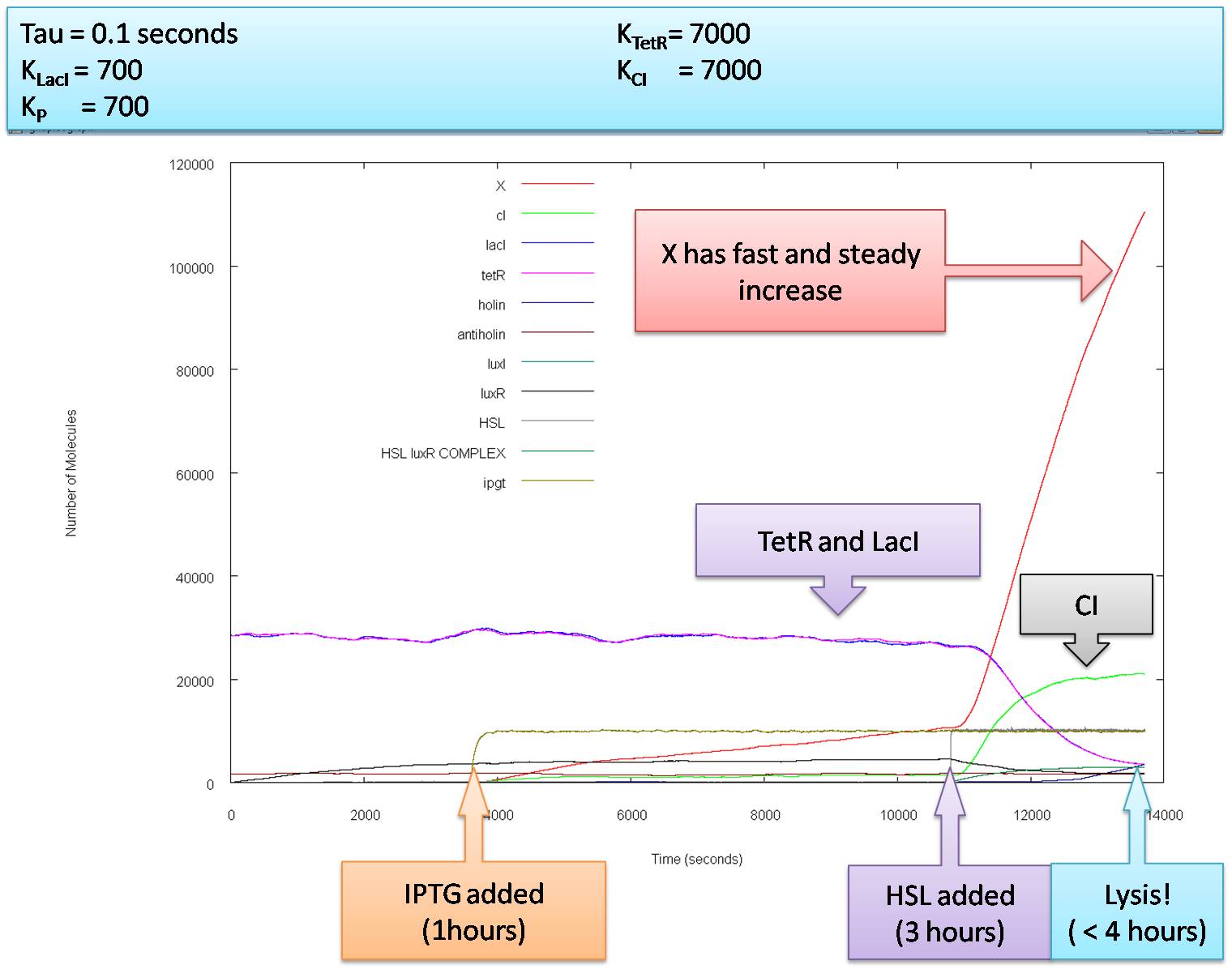
This process can be computationally very fast depending on the choice of tau. We ran several simulations to determine the dependence of the results on tau and found that the results were robust for tau between ~0.01 seconds and ~1.5 seconds. As expected, the larger tau is, the quicker the simulation runs. We see the comparison between tau = 0.01 seconds, tau = 0.1 seconds and tau =1.5 seconds below.
The three simulations with different tau timesteps yield almost identical results. We not however that the simulation results become non-meaningful for tau larger than 2s (results not shown here).
References
[1] Gillespie,
[2] T. Tian, K.Burrage, P. M. Burrage and M. Carletti (2006): Stochastic Delay Differential Equations for Genetic Regulatory Networks, Special Issue of J. Comp and Applied Maths, doi:10.1016/j.cam.2006.02.063
 "
"


