Team:USTC Software/WhatDemo
From 2009.igem.org
(→Mathematical Formulation) |
|||
| (22 intermediate revisions not shown) | |||
| Line 1: | Line 1: | ||
{{USTCSW_Heading}} | {{USTCSW_Heading}} | ||
| - | {|align = "justify" border = "1" bordercolor = "black" bgcolor = "red" | + | {|- |
| - | | | + | |valign = "top"| |
| - | '''Due to the incapaility of 2009.igem.org to interpret formula in Latex form to elligible expressions, we have to relink this page [https://igem.org/User:Heyu3/ | + | {{USTCSW_SideBarL}} |
| + | |align = "justify"| | ||
| + | {|- | ||
| + | |align = "justify" border = "1" bordercolor = "black" bgcolor = "red"| | ||
| + | '''Due to the incapaility of 2009.igem.org to interpret formula in Latex form to elligible expressions, we have to relink this page [https://igem.org/User:Heyu3/MM <font size = "4">HERE</font>]. This has been authorized by the organizers of iGEM. If you don't mind the formula part, you may still work with this page.''' | ||
| + | <br /> | ||
|} | |} | ||
| - | |||
| - | |||
| - | |||
| - | |||
| - | |||
| - | |||
| - | =Example 1. Synthetic Oscillator= | + | =Example 1. A Synthetic Oscillator= |
==Introduction== | ==Introduction== | ||
| Line 68: | Line 67: | ||
molecules increases. | molecules increases. | ||
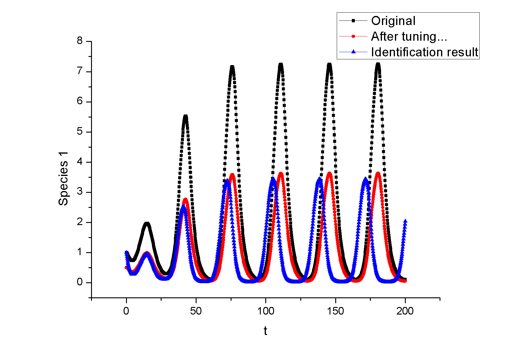
| - | [[ | + | [[Image:Osc1_Amp_Tun.png|center|550px|thumb|Tunable Amplitude: |
| + | The Black curve shows the original amplitude of the oscillator. | ||
| + | The Red curve shows the desired amplitude of the oscillator, | ||
| + | The blue curve is the identification result]] | ||
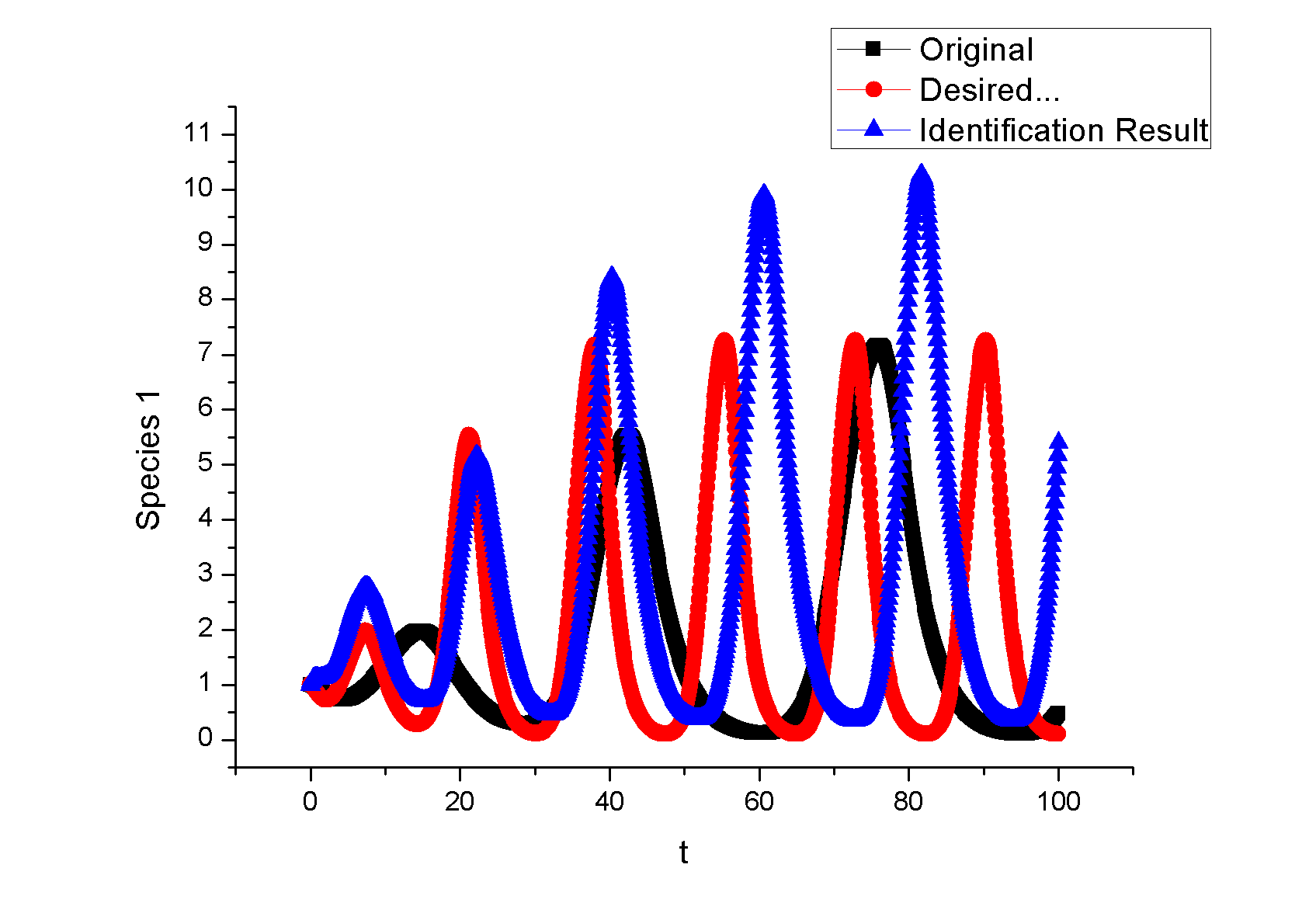
| - | [[ | + | [[Image:Osc1_Freq_Tun.png|center|550px|thumb|Tunable Frequency: |
| + | The Black curve shows the original frequency of the oscillator. | ||
| + | The Red curve shows the desired frequency of the oscillator, | ||
| + | The blue curve is the identification result]] | ||
==An Alternative Topology That Leads to Oscillation== | ==An Alternative Topology That Leads to Oscillation== | ||
| Line 86: | Line 91: | ||
\end{align}\,\!</math> | \end{align}\,\!</math> | ||
| - | [[ | + | [[Image:Osc2.png|center|550px|thumb|An Alternative Topology the leads to Oscillation]] |
| - | + | ||
| - | + | ||
| - | + | ||
=Example 2: Perfect Adaptation= | =Example 2: Perfect Adaptation= | ||
| Line 158: | Line 160: | ||
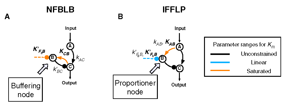
| - | Then we hope the output of interested node tracks the target dynamics by a sudden stimulus and search the feasible topologies that achieve adaptation in the scope of all possible topologies. | + | Then we hope the output of interested node tracks the target dynamics by a sudden stimulus and search the feasible topologies that achieve adaptation in the scope of all possible topologies. Two possible topologies are listed below: |
| - | [[ | + | [[ Image:Adaptation.png|center|550px|thumb|Two topologies that can achieve adaptation: Negative Feedback Loop with a Buffer Node (NFBLB) and Incoherent Feedforward Loop with a Proportioner Node (IFFLP) (Figure reproduced from [http://www.ncbi.nlm.nih.gov/pubmed/19703401 ''Defining Network Topologies that Can Achieve Biochemical Adaptation''])]] |
| - | + | ||
| - | [ | + | |
| - | + | ||
| - | + | ||
==Feedback loop== | ==Feedback loop== | ||
| Line 205: | Line 203: | ||
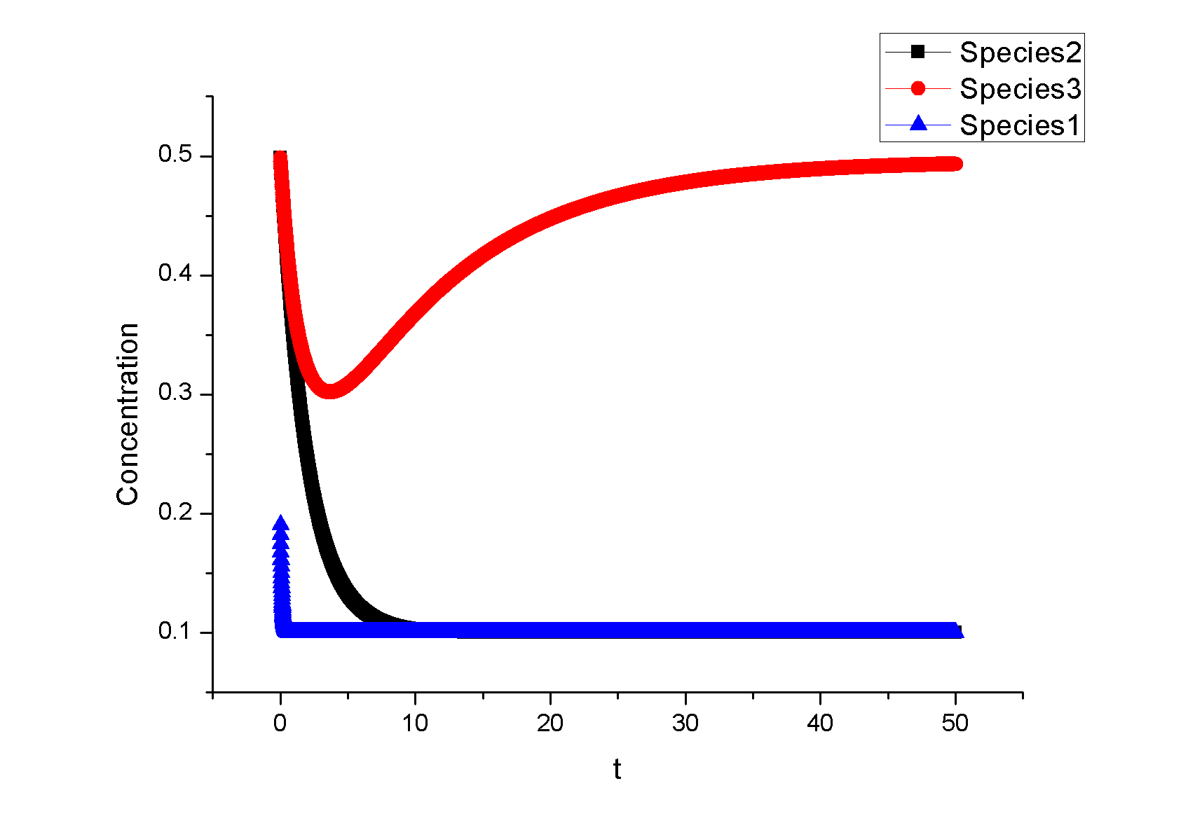
\\ \end{align}\,\!</math> | \\ \end{align}\,\!</math> | ||
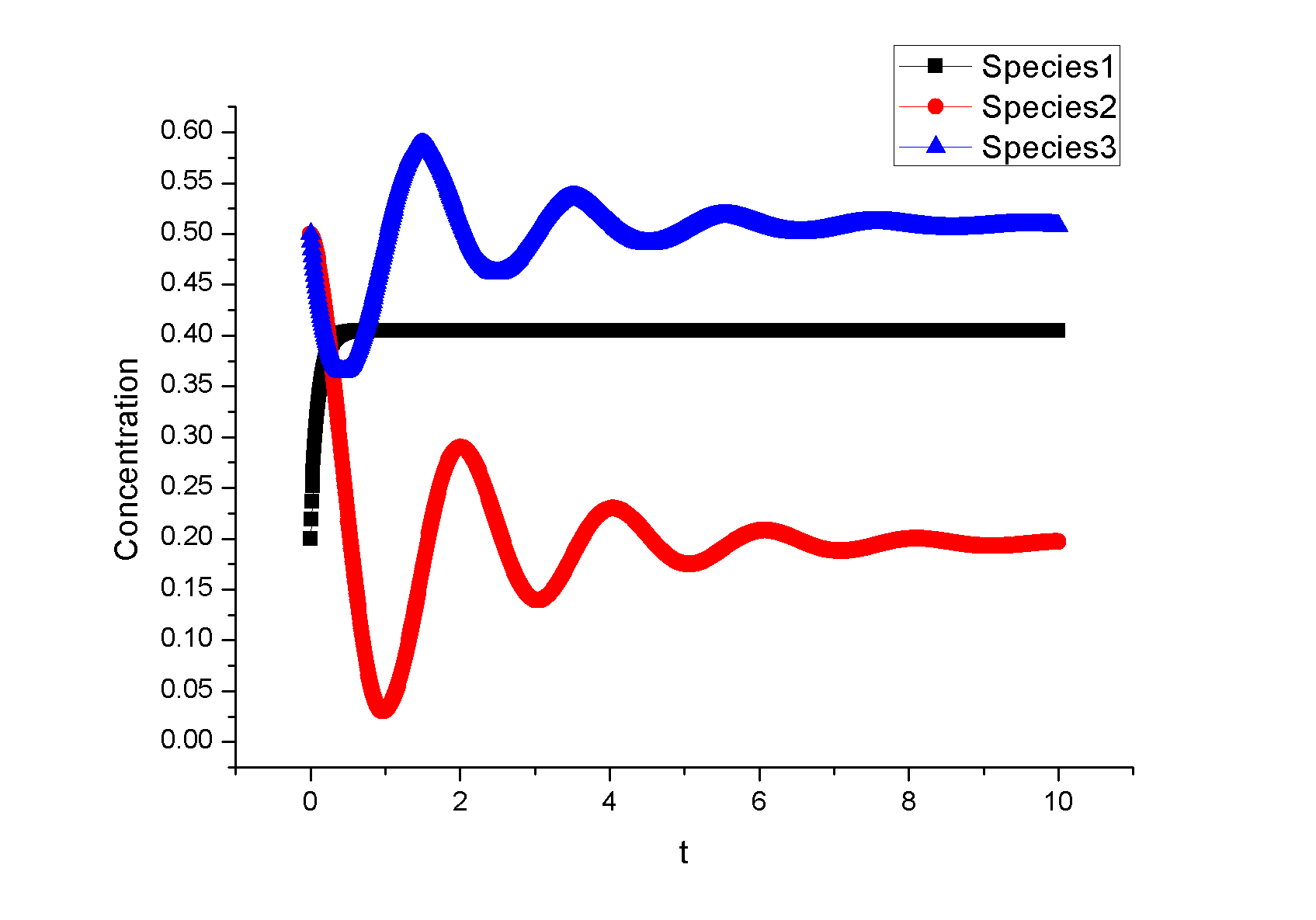
| - | [[ | + | [[ Image:Adapt2.png|center|550px|thumb|Simulation Result under stimulus 1]] |
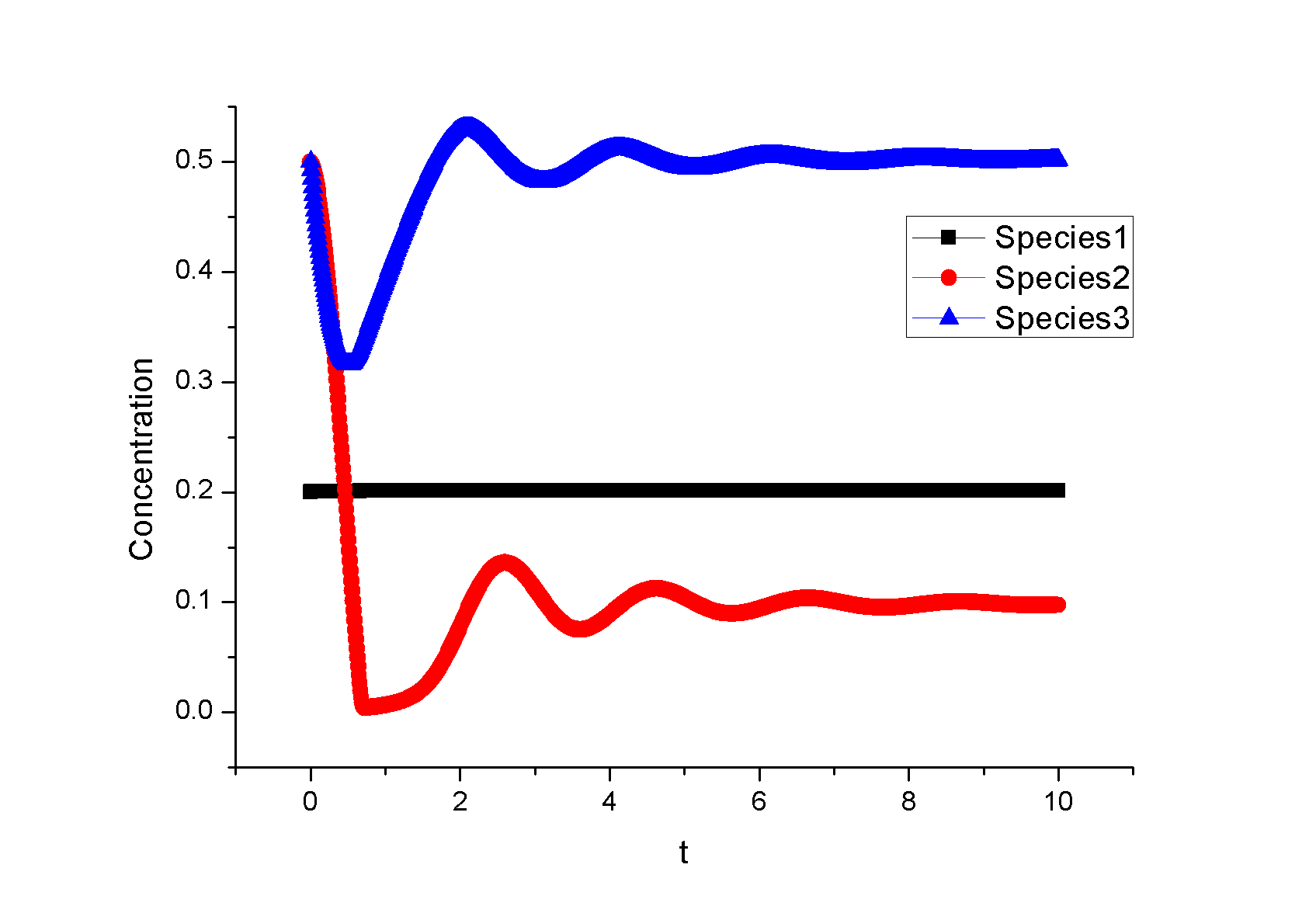
| - | [[ | + | [[Image:AdaptationSim1.png|center|550px|thumb|Simulation Result under stimulus 2]] |
| + | |||
| + | Global Sensitivity Analysis | ||
| + | We carry out global sensitivity analysis for this model, the result shows that | ||
| + | the sensitivity coefficient of stimilus is very small which also prove the | ||
| + | reliability of sensitivity analysis at the same time. | ||
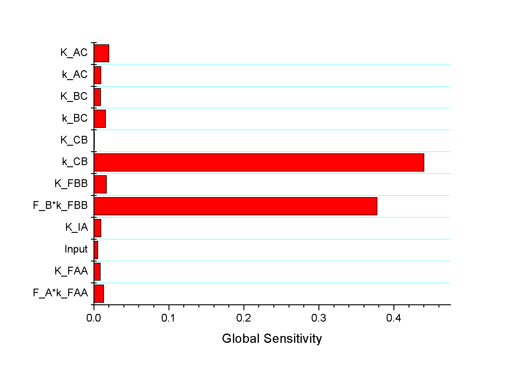
| + | The following figure shows global sensitivity coefficients | ||
| + | of 12 parameters in this system: | ||
| + | [[Image:Global_sensitivity.png|center|550px|thumb|global sensitivity coefficients | ||
| + | of 12 parameters in this system]] | ||
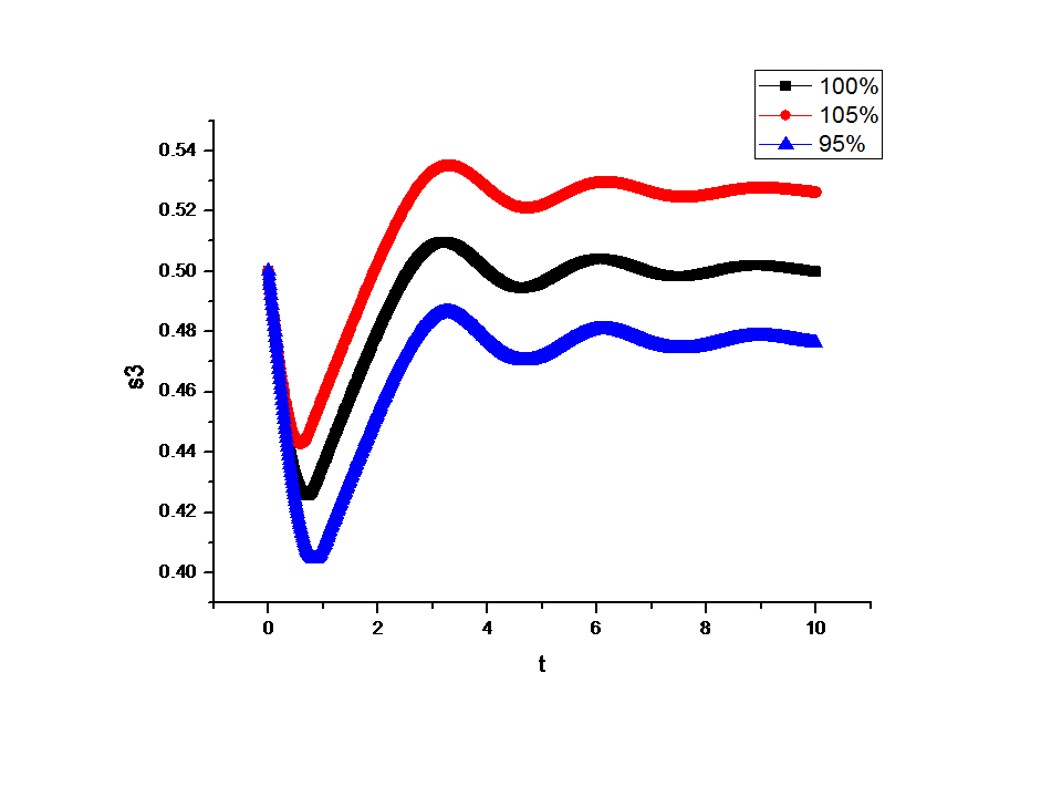
| + | Besides the external stimulus "input", we also check other two paramters. k_CB has the | ||
| + | greatest global senstivity value, we change its value by -5% and +5%, then simulate the | ||
| + | system again, the following figure shows change on species 3: | ||
| + | [[Image:SensKCB.png|center|550px|thumb|pertubation on species 3 after change of k_CB]] | ||
==Feedforward loop== | ==Feedforward loop== | ||
| Line 271: | Line 282: | ||
which can be independently tunedfrom the adaptation precision. | which can be independently tunedfrom the adaptation precision. | ||
| - | |||
| - | |||
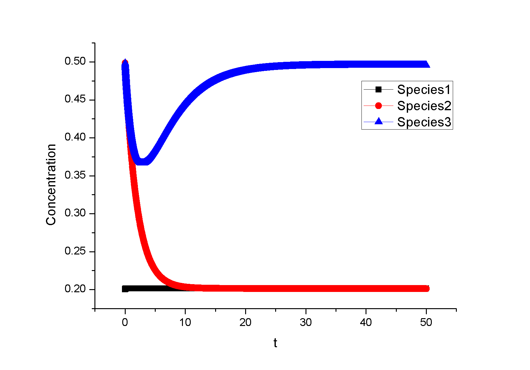
| - | + | [[ Image:AdaptFeedforward1.png|center|550px|thumb|Simulation Result under stimulus 1]] | |
| - | [[ | + | [[Image:AdaptFeedforward2.png|center|550px|thumb|Simulation Result under stimulus 2]] |
| - | + | ||
| - | + | ||
| - | + | ||
| - | + | ||
| - | + | ||
| - | + | ||
| - | + | ||
| - | + | ||
| - | + | ||
| - | + | ||
=Example 3. Bistable Toggle Switch= | =Example 3. Bistable Toggle Switch= | ||
| Line 335: | Line 334: | ||
assume that <math>\gamma =\theta =\eta =2</math> as parameter | assume that <math>\gamma =\theta =\eta =2</math> as parameter | ||
restriction. Thus, there are four parameters to be indentified. | restriction. Thus, there are four parameters to be indentified. | ||
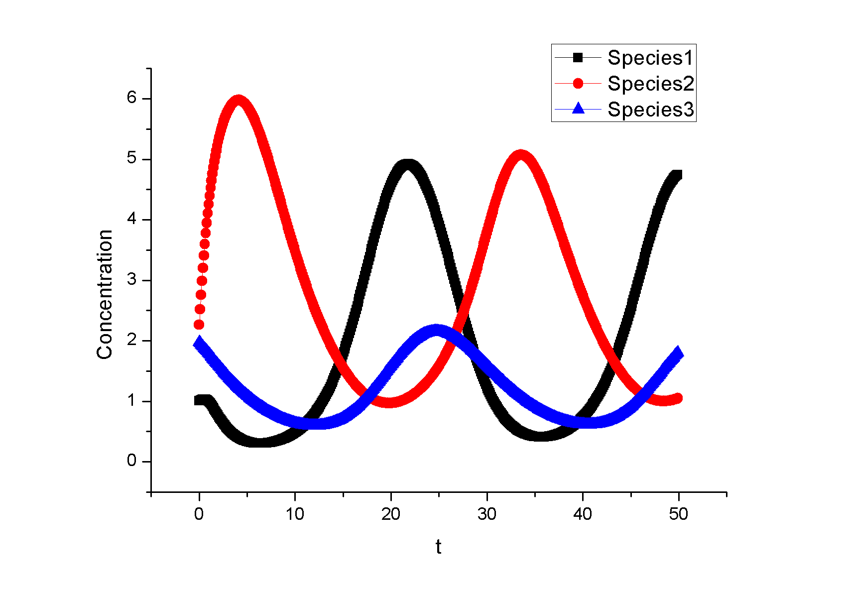
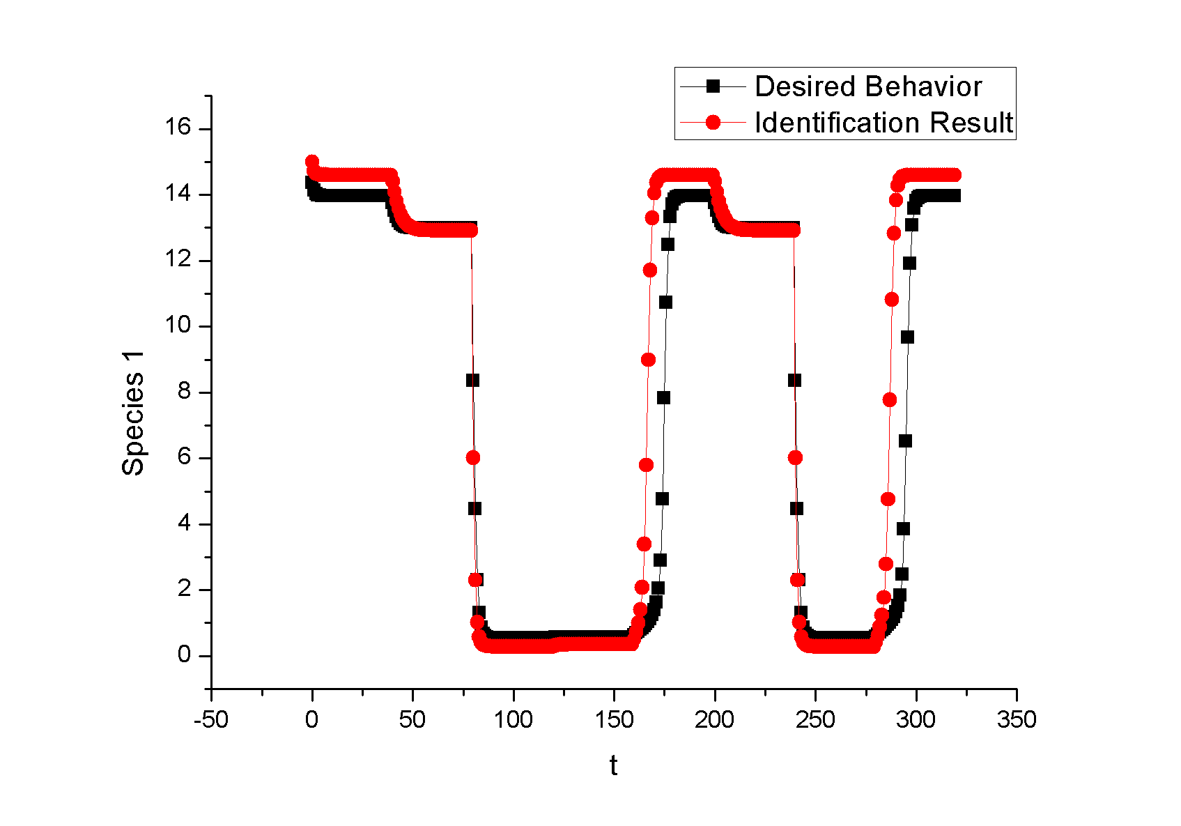
| + | [[Image:Toggle_Switch_Species1.png|center|550px|thumb|Identification Result | ||
| + | for the first species, the black curve is the desired behavior while the | ||
| + | red curve is the identification result]] | ||
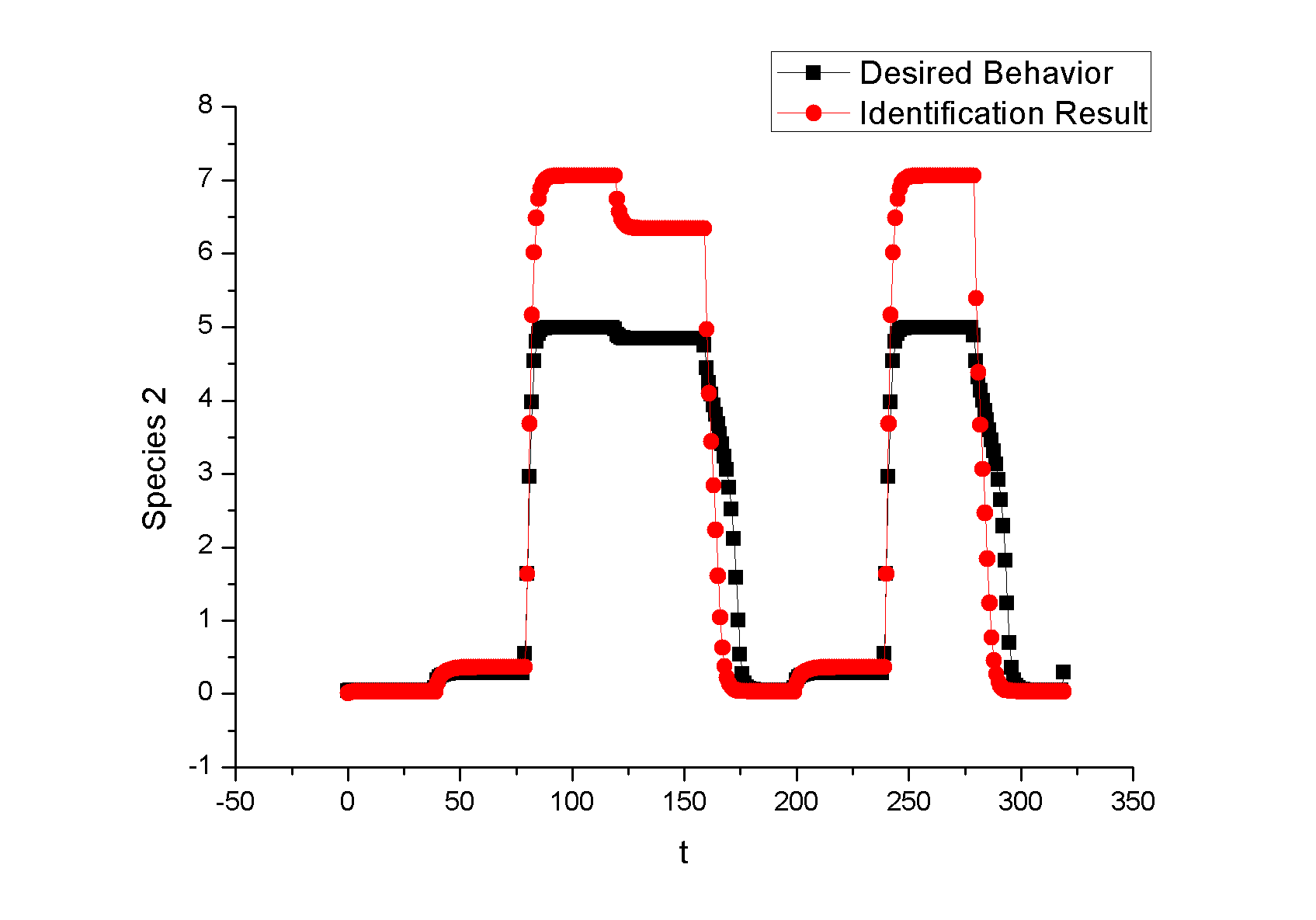
| + | [[Image:Toggle_Switch_Species2.png|center|550px|thumb|Identification Result | ||
| + | for the second species, the black curve is the desired behavior while the | ||
| + | red curve is the identification result]] | ||
| - | + | |valign = "top"| | |
| - | | | + | |
{{USTCSW_SideBarR}} | {{USTCSW_SideBarR}} | ||
|} | |} | ||
|} | |} | ||
{{USTCSW_Foot}} | {{USTCSW_Foot}} | ||
Latest revision as of 02:53, 22 October 2009
| About | Team and People | Project | Standard | Notebook | Demo | Safety | External Links |
|---|
|
|
Example 1. A Synthetic OscillatorIntroductionThe [http://www.ncbi.nlm.nih.gov/entrez/query.fcgi?cmd=Retrieve&db=pubmed&dopt=Abstract&list_uids=10659856&query_hl=2 synthetic oscillatory network] designed by [http://www.elowitz.caltech.edu/ Michael Elowitz] is pioneering work. In the first place, based on his model, we want to illustrate how to tune the parameters to get pre-defined wave amplitude and wave frequency. In the second place, besides this three node repressive model, is it possible to propose a alternative topology that could also achieve tunable oscillation. In [http://gardnerlab.bu.edu/ Tim Gardner]'s PhD dissertation, such a different topology is proposed. We search feasible parameter that could achieve oscillation. Mathematical FormulationThe activities of a gene are regulated by other genes through the interactions between them, i.e., the transcription and translation factors. Here, we assume that this system follows Hill kinetic law. <math>\begin{align} \frac{dm_{i}}{dt} &=-a_{i}m_{i}+\sum\limits_{j}b_{ij}\frac{p_{j}^{H_{ij}}}{K_{ij}+p_{j}^{H_{ij}}}+l_{i}, \\ \frac{dp_{i}}{dt} &=-c_{i}p_{i}+d_{i}m_{i}, (i=1,2,...,n) \end{align}\,\!</math> where <math>m_{i}(t), p_{i}(t)\in {\mathbb{R}}</math> are concentrations of mRNA and protein of the <math>i</math>th node at time <math>t</math>, respectively, <math>a_{i}</math> and <math>c_{i}</math> are the degradation rates of the mRNA and protein, <math>d_{i}</math> is the translation rate. Term (1) describes the transcription process and term (2) describes the translation process. Negative and positive signs of <math>b_{ij}</math> indicates the mutual interaction relationship that could be attributed to negative or positive feedback. The values describe the strength of promoters which is tunable by inserting different promoters in gene circuits. <math>H_{ij}</math> is Hill coefficient describing cooperativity. <math>K_{ij}</math> is the apparent dissociation constant derived from the law of mass action (equilibrium constant for dissociation). We can write <math>K_{ij}=\left( \hat{K}_{ij}\right) ^{n}</math> where <math>\hat{K}</math> is ligand concentration producing half occupation (ligand concentration occupying half of the binding sites), that is also the microscopic dissociation constant. A Tunable OscillatorThe original three repressors model is described as follows:% <math>\begin{align} \frac{dm_{1}}{dt} &=-am_{1}+b\frac{p_{3}^{H_{13}}}{K+p_{3}^{H_{1}}}, \\ \frac{dm_{2}}{dt} &=-am_{2}+b\frac{p_{1}^{H_{21}}}{K+p_{1}^{H_{2}}}, \\ \frac{dm_{3}}{dt} &=-am_{3}+b\frac{p_{2}^{H_{32}}}{K+p_{2}^{H_{32}}}, \\ \frac{dp_{1}}{dt} &=-cp_{1}+dm_{1}, \\ \frac{dp_{2}}{dt} &=-cp_{2}+dm_{2}, \\ \frac{dp_{3}}{dt} &=-cp_{3}+dm_{3},\text{ } \end{align}\,\!</math> where <math>a, b,</math> <math>c,</math> <math>d,</math> <math>H_{1},</math> <math>H_{2},</math> <math>H_{3},</math> <math>K</math> are tunable parameters that could change wave amplitude and frequency. For simplicity, we assume that <math>H_{13}=H_{21}=H_{32}=2,</math> meaning that the system contains only positively cooperative reaction that once one ligand molecule is bound to the enzyme, its affinity for other ligand molecules increases. An Alternative Topology That Leads to OscillationThe original three repressors model is described as follows:% <math>\begin{align} \frac{dm_{1}}{dt} &= -a_{1}x_{1}+\frac{b_{1}}{K_{1}+p_{2}^{H_{12}}}, \\ \frac{dm_{2}}{dt} &= -a_{2}x_{2}+\frac{b_{2}p_{3}^{H_{23}}}{% K_{2}+p_{1}^{H_{21}}+p_{3}^{H_{23}}}, \\ \frac{dm_{3}}{dt} &= -a_{3}x_{3}+\frac{b_{3}}{K_{3}+p_{2}^{H_{32}}} \\ \frac{dp_{1}}{dt} &= -c_{1}p_{1}+d_{1}m_{1}, \\ \frac{dp_{2}}{dt} &= -c_{2}p_{2}+d_{2}m_{2}, \\ \frac{dp_{3}}{dt} &= -c_{3}p_{3}+d_{3}m_{3}, \end{align}\,\!</math> Example 2: Perfect AdaptationIntroductionIn this example, we try to seek different network topologies that can achieve adaptation-the ability to reset themselves after responding to a stimulus.. Actually, most of the scripts are cited from a newly published paper on [http://www.cell.com/ Cell]: [http://www.ncbi.nlm.nih.gov/pubmed/19703401 Defining Network Topologies that Can Achieve Biochemical Adaptation]. It 's quite by accident that issues discussed in this paper share some similarities with our project. To test our ABCD is powerful or not, the only thing we need to do is to search the two topologies found in this paper. By running nearly two days, we prove the solution. Mathematical FormulationWe assume that each node (labeled as <math>A</math>, <math>B</math>, <math>C</math>) has a fixed concentration (normalized to <math>1</math>) but has two forms: active and inactive (here <math>A</math> represents the concentration of active state, and <math>1-A</math> is the concentration of the inactive state). The enzymatic regulation converts its target node between the two forms. For example, a positive regulation of node <math>B</math> by node <math>A</math> as denoted by a link <math>A\longrightarrow B</math> would mean that the active <math>A</math> convertsBfrom its inactive to its active form and would be modeled by the rate <math>R(B_{inactive}\longrightarrow B_{active})=k_{AB}A(1-B)/\left[ (1-B)+K_{AB}\right] </math>, where <math>A</math> is the normalized concentration of the active form of node <math>A</math> and <math>1-B</math> the normalized concentrations of the inactive form of node B. Likewise, <math>A-|B</math> implies that the active A catalyzes the reverse transition of node B from its active to its inactive form, with a rate <math>R(B_{active}\longrightarrow B_{inactive})=k_{AB}^{^{\prime }}/(B+K_{AB}^{^{\prime }}).</math> When there are multiple regulations of the same sign on a node, the effect is additive. For example, if node C is positively regulated by node A and node B, <math> R(C_{inactive}\longrightarrow C_{active})= k_{AC}A(1-C)/\left[ (1-C)+K_{AC}\right]</math> + <math>k_{BC}B(1-C)/\left[ (1-C)+K_{BC}\right] </math> . We assume that the interconversion between active and inactive forms of a node is reversible. Thus if a node <math>i</math> has only positive incoming links, it is assumed that there is a background (constitutive) deactivating enzyme Fi of a constant concentration (set to be <math>0.5</math>) to catalyze the reverse reaction. Similarly, a background activating enzyme <math>E_{i}=0.5</math> is added for the nodes that have only negative incoming links. The rate equation for a node (e.g., node <math>B</math>) takes the form: <math>\begin{align} \frac{dB}{dt}=\sum\limits_{i}X_{i}\cdot k_{X_{i}B}\frac{(1-B)}{ (1-B)+K_{X_{i}B}}-\sum\limits_{i}Y_{i}\cdot k_{X_{i}B}\frac{B}{B+K_{Y_{i}B}}, \\ \end{align}\,\!</math> where <math>Xi=A,B,C,E_{A},E_{B},</math> or <math>E_{c}</math> are the activating enzymes (positive regulators) of <math>B</math> and <math>Yi=A,B,C,F_{A},F_{B},</math> or <math>F_{C}</math> are the deactivating enzymes (negative regulators) of <math>B</math>. In the equation for node A, an input term is added to the righthand-side of the equation: <math> Ik_{IA}(1-A)/((1-A)+K_{IA})</math>. The number of parameters in a network is <math> n_{p}=2n_{I}+2</math>, where <math>n_{I}</math> is the number of links in the network (including links from the basal enzymes if present).
Feedback loopThe kinetic equations are as follows: <math>\begin{align} \frac{dA}{dt} &=&I\cdot k_{IA}\frac{(1-A)}{(1-A)+K_{IA}}-F_{A}\cdot k_{F_{A}A}^{^{\prime }}\frac{A}{A+K_{F_{A}A}^{^{\prime }}}, \\ \frac{dB}{dt} &=&C\cdot k_{CB}\frac{(1-B)}{(1-B)+K_{CB}}-F_{B}\cdot k_{F_{B}B}^{^{\prime }}\frac{B}{B+K_{F_{B}B}^{^{\prime }}}, \\ \frac{dB}{dt} &=&A\cdot k_{AC}\frac{(1-C)}{(1-C)+K_{AC}}-B\cdot k_{BC}^{^{\prime }}\frac{C}{C+K_{BC}^{^{\prime }}}, \\ \end{align}\,\!</math> where <math>F_{A}</math> and <math>F_{B}</math> represent the concentrations of basal enzymes that carry out the reverse reactions on nodes <math>A</math> and <math>B</math>, respectively (they oppose the active network links that activate <math>A</math> and <math>B</math>). In this circuit, node <math>A</math> simply functions as a passive relay of the input to node <math>C</math>; the circuit would work in the same way if the input were directly acting on node <math>C</math> (just replacing <math>A</math> with <math>I</math> in the third equation of Equation 1). Analyzing the parameter sets that enabled this topology to adapt indicates that the two constants <math>K_{CB}</math> and <math>K_{F_{B}B}^{^{\prime }}</math> (Michaelis-Menten constants for activation of <math>B</math> by <math>C</math> and inhibition of <math>B </math> by the basal enzyme) tend to be small, suggesting that the two enzymes acting on node <math>B</math> must approach saturation to achieve adaptation. Indeed, it can be shown that in the case of saturation this topology can achieve perfect adaptation. <math>\begin{align} \begin{tabular}{l} </math>figure\text{ 1}\text{: desired input}</math> \\ </math>figure\text{ 2}\text{: different inputs}</math> \\ </math>figure\text{ 3: }</math>topology \end{tabular} \\ \end{align}\,\!</math> Global Sensitivity Analysis We carry out global sensitivity analysis for this model, the result shows that the sensitivity coefficient of stimilus is very small which also prove the reliability of sensitivity analysis at the same time. The following figure shows global sensitivity coefficients of 12 parameters in this system: Besides the external stimulus "input", we also check other two paramters. k_CB has the greatest global senstivity value, we change its value by -5% and +5%, then simulate the system again, the following figure shows change on species 3: Feedforward loopThe kinetic equations are as follows: <math>\begin{align} \frac{dA}{dt} &=&I\cdot k_{IA}\frac{(1-A)}{(1-A)+K_{IA}}-F_{A}\cdot k_{F_{A}A}^{^{\prime }}\frac{A}{A+K_{F_{A}A}^{^{\prime }}}, \\ \frac{dB}{dt} &=&A\cdot k_{AB}\frac{(1-B)}{(1-B)+K_{AB}}-F_{B}\cdot k_{F_{B}B}^{^{\prime }}\frac{B}{B+K_{F_{B}B}^{^{\prime }}}, \\ \frac{dB}{dt} &=&A\cdot k_{AC}\frac{(1-C)}{(1-C)+K_{AC}}-B\cdot k_{BC}^{^{\prime }}\frac{C}{C+K_{BC}^{^{\prime }}}, \\ \end{align}\,\!</math> The adaptation mechanism is mathematically captured in the equation for node <math>C</math>: if the steady-state concentration of the negative regulator B is proportional to that of the positive regulator <math>A</math>, the equation determining the steady-state value of <math>C</math>, <math>dC/dt=0</math>, would be independent of <math>A</math> and hence of the input <math>I</math>. In this case, the equation for node <math>B</math> generates the condition under which the steady-state value <math> B^*</math> would be proportional to <math>A^*</math>: the first term in <math>dB/dt</math> equation should depend on <math>A</math> only and the second term on <math>B</math> only. The condition can be satisfied if the first term is in the saturated region region <math>((1-B)\gg K_{AB})</math> and the second in the linear region <math>B\ll K_{F_{B}B}^{^{\prime }}</math>, leading to <math>\begin{align} B^{\ast }=A^{\ast }\cdot k_{AB}K_{F_{B}B}^{^{\prime }}/(F_{B}k_{F_{B}B}^{^{\prime }}) \\ \end{align}\,\!</math> This relationship, established by the equation for node <math>B</math>, shows that the steady-state concentration of active <math>B</math> is proportional to the steady-state concentration of active <math>A</math>. Thus <math>B</math> will negatively regulate <math>C</math> in proportion to the degree of pathway input. This effect of <math>B</math> acting as a proportioner node of <math>A</math> can be graphically gleaned from the plot of the <math>B</math> and <math>C</math> nullclines (Figure feedforward). In this case, maintaining a constant <math>C^{\ast }</math> requires the B nullcline to move the same distance as the <math>C</math> nullcline in response to an input change. Here again, the sensitivity of the circuit (the magnitude of the transient response) depends on the ratio of the speeds of the two signal transduction branches: <math> A\longrightarrow C</math> and <math>A\longrightarrow B-|C</math>, which can be independently tunedfrom the adaptation precision.
Example 3. Bistable Toggle SwitchIntroductionA good example of engineering in Synthetic Biology include the pioneering work of [http://gardnerlab.bu.edu/ Tim Gardner] and [http://www.bu.edu/abl/ James Collins] on an [http://www.ncbi.nlm.nih.gov/entrez/query.fcgi?cmd=Retrieve&db=pubmed&dopt=Abstract&list_uids=10659857&query_hl=5 engineered genetic toggle switch]. Here, we want to show how to tune parameters to guarantee bistability. Mathematical Formulation<math>\begin{align} \dot{u}(t) &=\frac{\alpha _{1}}{1+v^{\theta }(t)}-\beta _{1}u(t), (.....................................equation1) \\ \dot{v}(t) &=\frac{\alpha _{2}X^{\eta }}{X^{\eta }+1+u^{\gamma }(t)}-\beta _{2}v(t),(..............................................equation2) \\ \end{align}\,\!</math> where <math>X</math> is input, <math>u</math> is the concentration of repressor 1, <math>v</math> is the concentration of repressor 2, <math>\alpha _{1}</math> is the effective rate of synthesis of repressor 1, <math>\alpha _{2}</math> is the effective rate of synthesis of repressor 2, <math>\theta </math> is the cooperativity of repression of promoter 2 and <math>\gamma </math> is the cooperativity of repression of promoter 1. The above model is derived from a biochemical rate equation formulation of gene expression. The final form of the toggle equations preserves the two most fundamental aspects of the network: cooperative repression of constitutively transcribed promoters (the first term in each equation), and degradation/dilution of the repressors (the second term in each equation). The parameters <math>\alpha _{1}</math> and <math>\alpha _{2}</math> are lumped parameters that describe the net effect of RNA polymerase binding, open-complex formation, transcript elongation, transcript termination, repressor binding, ribosome binding and polypeptide elongation. The cooperativity described by <math>\theta </math> and <math>\gamma </math> can arise from the multimerization of the repressor proteins and the cooperative binding of repressor multimers to multiple operator sites in the promoter. An additional modification to equation (1) is needed to describe induction of the repressors. <math>\alpha _{1},\alpha _{2},\gamma ,\theta ,\eta ,\beta _{1},\beta _{2}</math> should be indentified to guarantee bistability. We assume that <math>\gamma =\theta =\eta =2</math> as parameter restriction. Thus, there are four parameters to be indentified. |
|
 "
"


