Team:USTC/Modeling/Model-2
From 2009.igem.org
| (8 intermediate revisions not shown) | |||
| Line 18: | Line 18: | ||
| - | [[Image:sm2-1-1- | + | [[Image:sm2-1-1-3.jpg|900px]] |
| - | From above equations, we can the change of PoPS respond to the AHL<sub>in</sub>. | + | From above equations, we can estimate the change of PoPS respond to the AHL<sub>in</sub>. |
| Line 27: | Line 27: | ||
| - | For | + | For this system, the value of parameter d, 0.00847, could be estimated based on the measurement of the OD. For instance, when the concentration of AHL<sub>out</sub> was zero, the value of d was 0.00368 per minute. The values of 4.8E-3 per sec for rmG, 1.8E-3 per sec for a and 0.4 per sec for pG were got from the experiment conducted by Barry Canton and Anna Labno in 2004, click [http://partsregistry.org/Part:BBa_F2620:Experience/Endy/Data_analysis here] to the details. |
| - | [[Image:SM2-3.jpg|450px]] | + | [[Image:SM2-3.jpg|450px|center]] |
| - | With the help of [https://2009.igem.org/Team:USTC_Software USTC_Software], we succeeded to estimate the values of k<sub>3</sub>, r<sub>AHLin</sub>, C<sub>1</sub>, C<sub>2</sub>, C<sub>3</sub> and C<sub>4</sub>. The simulation results as follows. | + | With the help of [https://2009.igem.org/Team:USTC_Software USTC_Software], we succeeded to estimate the values of k<sub>3</sub>, r<sub>AHLin</sub>, C<sub>1</sub>, C<sub>2</sub>, C<sub>3</sub> and C<sub>4</sub>, using the data from our measurements. The simulation results as follows. |
k3=0.8; rAHL=0.001; | k3=0.8; rAHL=0.001; | ||
C1=1.5*10^(-10); C2=1*10^(10); C3=8*10^(-7); C4=5.8*10^(11) | C1=1.5*10^(-10); C2=1*10^(10); C3=8*10^(-7); C4=5.8*10^(11) | ||
| - | [[Image:sm2-4.jpg|800px]] | + | [[Image:sm2-4.jpg|800px|center]] |
| - | In | + | In above picture, the dots were the measuring poingts in our system and the curves were the corresponding simulations to a particular concentration of AHL<sub>out</sub>. |
| + | |||
| + | |||
| + | [[Image:sm2-5.jpg|center]] | ||
| + | |||
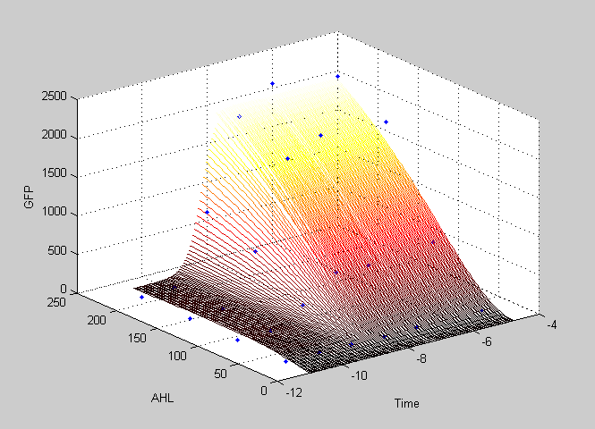
| + | In above picture, the dots were the measuring poingts in our system and the surface was the corresponding simulation. | ||
Latest revision as of 03:23, 22 October 2009
| Home | Team | Project | Modeling | Parts | Standard & Protocol | Software Tool | Human Practice | Notebook |
|---|
Team:USTC/Modeling/Model-2
Contents |
pConX2+LuxR+pLux/Tet+GFP
Parts:
Simplified Model-2
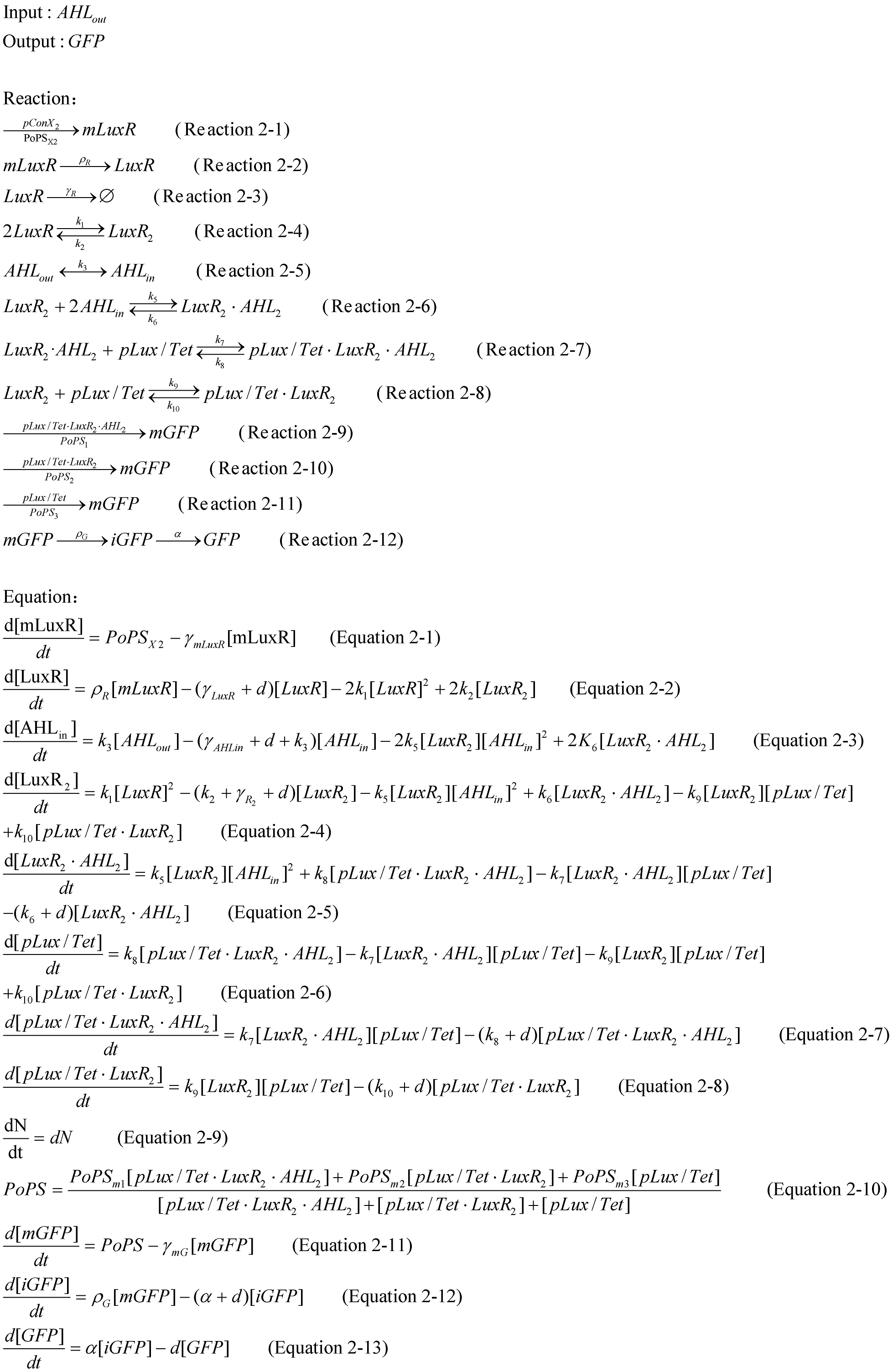
We employed an ODE model. We defined the input to be AHLout the and the output to be the synthesis rate of mature GFP. In this system,we assumed the concentration of the LuxR was constant.
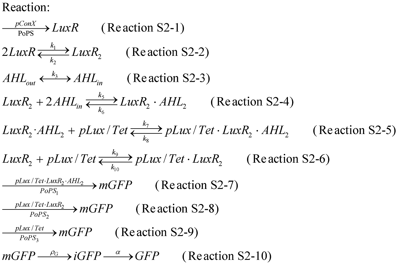
To simplify the model, the (Recation S2-4), (Recation S2-5) and (Recation S2-6) were considered to be able to get balance in a very short time.
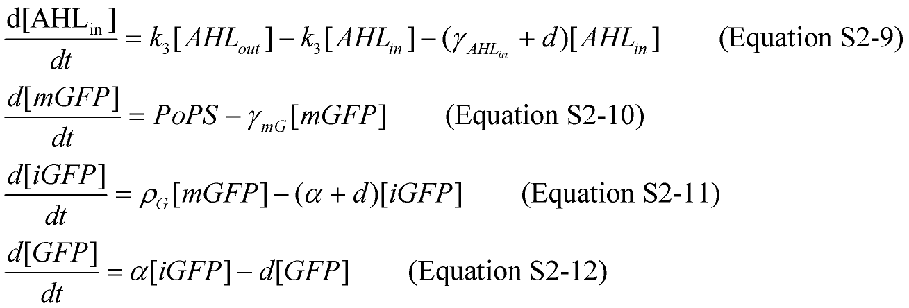
From above equations, we can estimate the change of PoPS respond to the AHLin.
For this system, the value of parameter d, 0.00847, could be estimated based on the measurement of the OD. For instance, when the concentration of AHLout was zero, the value of d was 0.00368 per minute. The values of 4.8E-3 per sec for rmG, 1.8E-3 per sec for a and 0.4 per sec for pG were got from the experiment conducted by Barry Canton and Anna Labno in 2004, click [http://partsregistry.org/Part:BBa_F2620:Experience/Endy/Data_analysis here] to the details.
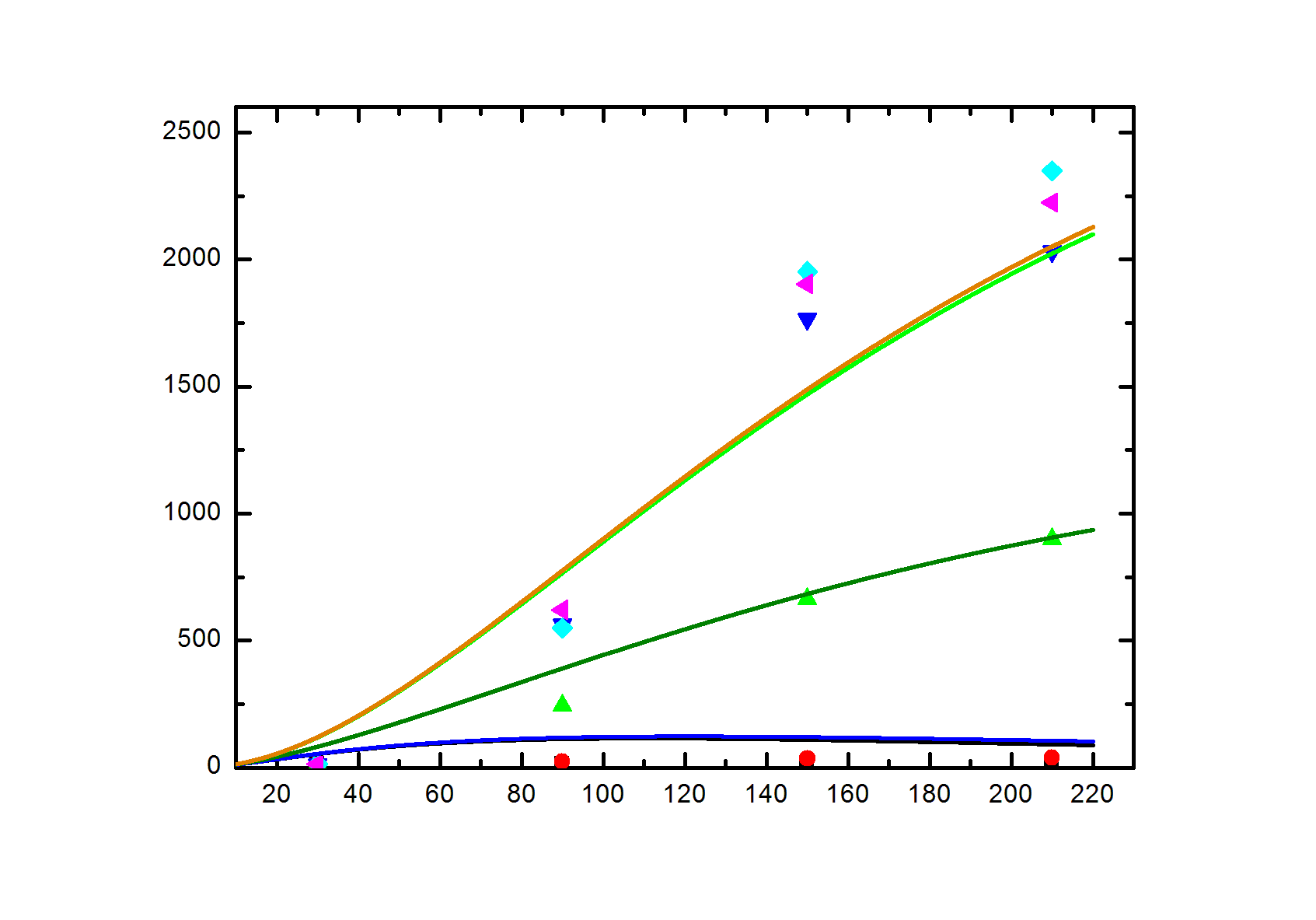
With the help of USTC_Software, we succeeded to estimate the values of k3, rAHLin, C1, C2, C3 and C4, using the data from our measurements. The simulation results as follows.
k3=0.8; rAHL=0.001; C1=1.5*10^(-10); C2=1*10^(10); C3=8*10^(-7); C4=5.8*10^(11)
In above picture, the dots were the measuring poingts in our system and the curves were the corresponding simulations to a particular concentration of AHLout.
In above picture, the dots were the measuring poingts in our system and the surface was the corresponding simulation.
 "
"

