Team:USTC Software/hoWMMD

Mathematical Formulation

High dimensional model representation(HDMR) is a general set of quantitative model assessment and analysis tools for capturing high dimensional IO system behavior. As the impact of the multiple input variables on the output can be independent and cooperative, it is natural to express the model output ()fx as a finite hierarchical correlated function expansion in terms of the input variables:

<math>\begin{align} f(x)& =f_{0}+\sum_{i=1}^{n}f_{i}(x_{i})+\sum_{1\leq i<j\leq n} f_{ij}(x_{i}, x_{j})+ \sum_{1\leq i<j<k\leq n}f_{ijk}(x_{i},x_{j},x_{k})+...+\sum_{1\leq i_{1}<...<i_{l}\leq n}f_{i_{1}i_{2}...i_{l}}(x_{i1},x_{i2},...,x_{il}) +...+f_{12...n}(x_{1},x_{2},...,x_{n})\\ \end{align}\,\!</math>

where the zeroth-order component function <math>f_{0}</math> is a constant representing the mean response to <math>f(x)</math>, and the first order component function <math>% f_{i}(x_{i})</math> gives the independent contribution to <math>f(x)</math> by the ith input variable acting alone, the second order component function <math>f_{ij}(x_{i},x_{j})</math> gives the pair correlated contribution to <math>f(x)</math> by the input variables <math>x_{i}</math> and <math>x_{j}</math>, etc. The last term contains any residual <math>n</math>th order correlated contribution of all input variables.

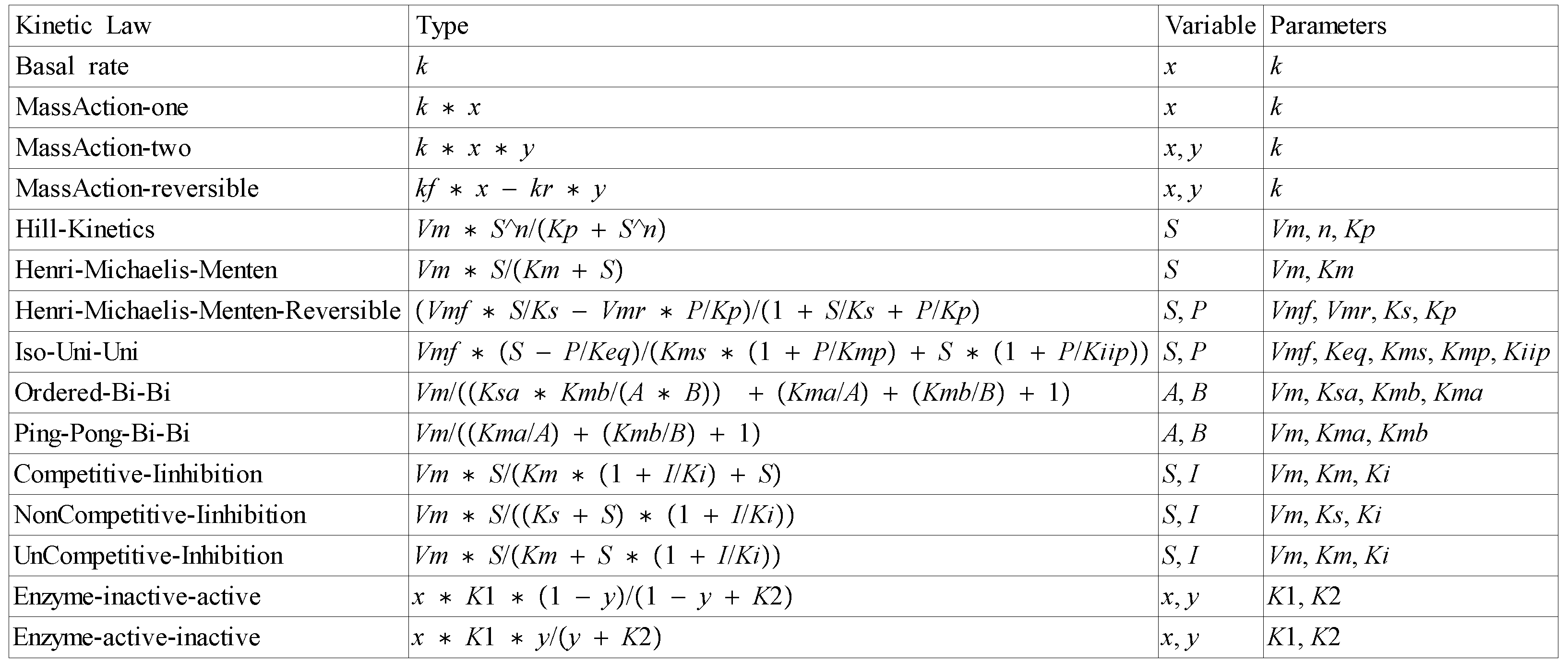
The basic conjecture underlying HDMR is that the component functions arising in typical real problems are likely to exhibit only low order l cooperativity among the input variables such that the significant terms in the HDMR expansion are expected to satisfy the relation: <math>l\ll n</math> for <math>n\gg 1 </math>. An HDMR expansion to second order

<math>\begin{align} f(x)=f_{0}+\sum\limits_{i=1}^{n}f_{i}(x_{i})+\sum\limits_{1\leq i<j\leq n}f_{ij}(x_{i},x_{j}), \\ \end{align}\,\!</math>

often provides a satisfactory description of <math>f(x)</math> for many high dimensional systems when the input variables are properly chosen. This is also the formula we use to achieve HDMR expansion. Similarly, reactants of two at most are usually involed in biochemical reactions. Thus, we can simplify the differential equations to the following form:

<math>\begin{align} \frac{dx_{k}}{dt} &=&\sum\limits_{i=1}^{n}f_{i}(x_{i},{\mathbf{p}} _{i})+\sum\limits_{1\leq i<j\leq n}f_{ij}(x_{i},x_{j},{\mathbf{p}} _{ij})-kx_{i}+C_{k}\\ \end{align}\,\!</math>

<math>\begin{align}s.t.\text{ algebra equations} \\ \end{align}\,\!</math>

for <math>k=1,\ldots ,n.</math> The left side term of the equation above represents the changing rate of variable <math>x_{k}.</math>We assume that each term on the right side represents one step biochemical reaction which is equivalent to the rate term defined in SBML. It means that changing rate of one variavle is determined by different rate terms. <math>C_{k}</math> is a constant number. <math>f_{i}(\cdot )</math> and <math>f_{ij}(\cdot )</math> have similar definitions and represent reaction rates that vary according to kinetic laws. <math>{\mathbf{p}}_{i}</math> and <math>{% \mathbf{p}}_{ij}</math> contain the parameter values of the kinetic law. It should mention that the last term\ <math>-kx_{i}</math>\ represents the degradation of <math>x_{i},</math>\ which seems to belong to <math>f_{i}(x_{i})</math> that\ may render degradation term undermined, we should add such a term for its ubiqutious existence in biological systems.

It is illustrative to consider the network generation task using a compact mathematical framework. Especially for metabolic networks, the structural and kinetic information can be well summarized using a time variant concentration vector <math>\mathbf{x}</math>, a time invariant stoichimetric matrix <math>S</math>% , and a time variant reaction rate vector <math>\mathbf{v}</math>. Vector <math>v</math> contains concentrations for all the <math>k</math> species <math>(x_{k},k=1,...,n)</math>. The <math>n\times m</math> matrix <math>S</math> represents the network structure by storing stoichiometric coefficients of all n reactions in its columns. The element <math>S(i,j)>0</math> if reaction <math>j</math> produces species <math>i</math>, <math>S(i,j)<0</math> if reaction <math>j</math> consumes species <math>i</math>, and otherwise <math>S(i,j)=0</math>. The reaction rate vector <math>\mathbf{v}</math> describes reaction rates <math>v_{j}</math>, <math>j=1,...,n</math>. Reaction rates vary according to kinetic laws which are linear or nonlinear algebraic functions.

Typically, kinetic laws determine the rates based on the amounts of species participating to reactions as well as various reaction specific parameters. Altogether, an ODE model can be formulated as

<math>\begin{align} \frac{d\mathbf{x}}{dt}=S\mathbf{v} \\ \end{align}\,\!</math>

The reaction rates <math>v_{j}</math>, <math>j=1,...,m</math> are determined by kinetic laws <math>f_{j} </math> as%

<math>\begin{align} v_{j}=f_{j}({\mathbf{x}}_{j},{\mathbf{p}}_{j}), \\ \end{align}\,\!</math>

in which <math>{\mathbf{x}}_{j}</math> includes concentrations of species taking part in the reaction <math>j</math>, and <math>{\mathbf{p}}_{j}</math> contains the parameter values of the kinetic law.

Candidate Kinetic Laws

Inspired by Matlab SimBiology (The MathWorks™), we list possible kinetic laws that are mostly encountered in biochemical reactions. These candidate kinetic laws are utilized in design sub level 1,2,3 and will be shuffled in GA.

Candidate Kinetic Law Table