Team:UAB-Barcelona/Modeling

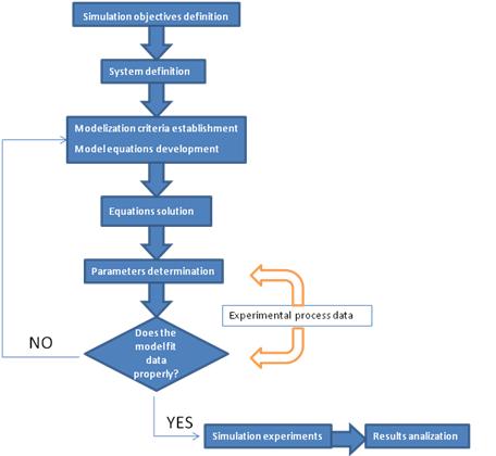
What is a model?

The answer will differ among communities of researchers. In the broadest sense, a model is an abstract representation of objects or processes that explains features of these objects or processes. Is important to remember that we are not only going to assign a model, we are going to simulate it as well to see if it explains the real biological process.

Steps to succes modelizing a system

Assumptions

Probably the most vital role that the modeler plays in modeling is in exercising his scientific judgment as to what assumptions can be validly made. Obviously an extremely rigorous model that includes every phenomenon down to microscopic detail would be so complex that it would take a long time to develop and might be impossible to solve. A modeling compromise between a rigorous description and getting an answer that is good enough is always required. This has been called “optimum sloppiness”. It involves making as many simplifying assumptions as are optimum usually corresponds to a model which is as complex as the available computing facilities will permit. The assumptions that are mode should be carefully considered and listed. They impose limitations on the model that should always be kept in mind when evaluating its predicted results.

Model Assignment is not Unique

Biological phenomena can be described in mathematical terms. It is important to note that a certain process can be described in more than one way.

• A biological object can be investigated with different experimental methods.

• Each biological process can be described with different (mathematical) models.

• A mathematical formalism may be applied to different biological instances.

• The choice of a mathematical model or an algorithm to describe a biological object depends on the problem, the purpose, and the intention of the investigator.

• Modeling has to reflect essential properties of the system. Different models may highlight different aspects of the same instance.

This ambiguity has the advantage that different ways of studying a problem also provide different insights into the systems. An important disadvantage is that the diversity of modeling approaches makes it very difficult to merge established models.

Stochastic Processes

The use of differential equations for describing biochemical processes makes certain assumptions that are not always justified. One assumption is that variables can attain continuous values. This is obviously a simplification, since the underlying biological objects, molecules, have discrete nature. As long as molecule numbers are sufficiently large this is no problem, but if the involved molecule numbers are only on the order of dozens or hundreds, the discreteness should be taken into account. Another important assumption of differential equations is that they treat the described process as deterministic. Random fluctuations are normally not part of differential equations. Again, this presumption does not hold for very small systems. A solution to both limitations is to use stochastic simulation approach that explicitly calculates the change of the number of molecules of participating species during the time course of a chemical reaction.

Steady States

The concept of stationary states is important for the modeling of dynamical systems. Stationary states are determined by the fact that the values of all state variables remain constant in time. The asymptotic behavior of dynamic systems is often stationary. The consideration of steady states is actually an abstraction that is based on a separation of time scales. While fast processes often reach a quasi-steady state after short transition period, the change of the value of the slow variables is often negligible in the time window of consideration. Thus each steady state can be regarded as a quasi-steady state of a system that is embedded in a larger non-stationary environment. Although the concept of stationary states is a mathematical idealization, it is important in kinetic modeling since it points to typical behavioral modes of investigated system and the respective mathematical problems are frequently easier to solve.

Modeling global transcription

The activity of every bacterial gene depends on the concentration of free RNA polymerase, [Rf], and on the promoter-specific Michaelis-Menten parameters, Vmax and Km, that determine the RNA polymerase-promoter interaction during transcript initiation [1]. Generally constitutive promoters are distinguished from regulated promoters; for the first, Vmax and Km remain constant under varying conditions of growth, whereas for the latter, Vmax and/or Km vary.

EFFECT OF THE FREE RNA POLYMERASE ON THE RATE OF TRANSCRIPTION INITIATION AT A GIVEN PROMOTER

All mathematical relationships involving free RNA polymerase derived below refer to steady-state conditions in exponentially growing bacterial cultures and are based on the standard Michaelis-Menten equation:

Transcription kinetics 1

Here V is the rate of transcript initiation at a given promoter, [Rf] is the concentration of free functional RNA polymerase, Vmax is the maximum rate of initiation at saturation of the promoter with RNA polymerase, and Km is the free RNA polymerase concentration that produces the half maximal rate.

EFFECT OF FREE RNA POLYMERASE ON THE RATE OF TRANSCRIPTION FROM A GIVEN PROMOTER

The rate of transcription, ri, originating from a given promoter Pi with an associated length of transcripts, Li, equals the product of the initiation rate V, given by the equation written before, the transcript length:

Transcription kinetics 2

If V and Vmax are measured as initiations per minute per promoter and the length of transcripts is measured in nucleotides, then ri is obtained as RNA nucleotides polymerized per min during steady-state expression from the promoter Pi. From this it is clear that ri is proportional to [Rf] only if the free RNA polymerase concentration is much smaller than Km.

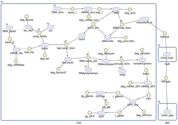
INTRODUCTION

A mathematical model of the detection and degradation of chloroform by a recombinant Escherichia Coli is proposed. The model includes chloroform transport to the cell, transport to the gas phase, transformation and output (GFP) induction. Our model consist of a system of seventeen nonlinear ordinary differential equations describing the temporal evolution of the key variables involved in the regulation of the pathway mentioned before. Computational simulations of our model are carried out for different external concentration of chloroform.

REACTIONS

To check which reactions take place in our model and the kinetic laws assumed for all of them, please download the following file. Here you will find a table summing up all that information.

PARAMETERS

The values of the coefficients used and the reference where they were taken are detailed in the next file.

In the absence of reliable experimental data, we chose some of our parameters based on expected reaction times and reactions equilibriums. Some others were taken from the bibliography cited at the end of this work. Although our simulations show that qualitative behavior of the solutions is similar for a large range of parameters. Therefore, we present here results obtained for the particular choice of parameters.

Ordinary Differential Equations (ODE's)