Team:Uppsala-Sweden/Modelling
From 2009.igem.org

Modelling of Ethanol Production
For our modell we have some basic assumptions that are
1. Co-evolution of the of the ethanol producing pathway, making km and kcat being highly similar for pdc as well as ADH. This assumption makes it possible for us to model the system as a single step reaction from pyruvate to ethanol. Greatly increasing the ease of simulation.
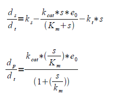
2. Assuming quasi steady state (Michaelis Menten Kinetics), that is constant total enzyme concentration. This is reasonable during log-phase before ethanol starts to inhibit growth.
Where e is the amount of free enzyme and es is the amount of enzyme bound to substrate.
Where ks is the rate of substrate formation (flux of the glycolysis), kcat is the maximum number of enzymatic reactions catalyzed per second, kt is the rate constant for the loss of substrate to other pathways, in our case primarily to the Krebbs cycle, Km is the substrate concentration at half the maximum reaction rate (Vmax) and s is the substrate concentration.
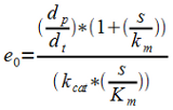
Having the Km and Kcat values gives e0 from the level of product formation.
3. Having e0 and letting kt go towards zero gives ks. kt can be assumed to approach zero provided that the Krebbs cycle is the main native consumer of pyruvate and that the inhibition of the PDC is successful. Gives a rearranged equation (b).
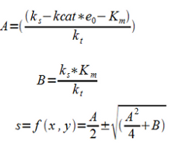
4. Assuming ks to be constant within the interval and assuming steady-state (ds/dt = 0) and rearranging to a 2:nd degree equation.
S is a function of f(x,y) where x is proportional to e0 and y is proportional to kt through the fitting constants A and B which are determined by measuring the substrate (pyruvate) concentration at different levels of enzyme concentration and inhibition of the PDC. In other words this correlates with the activity of efficiency of the promoters for the ethanol construct and the PDC inhibiting construct. These are then the two factors we can change in the system by using two different inducible promoters.
Measure for different x and y (activity of the two promoters) and fit the function to data through A and B.
This give us the final expression for product levels dependent only on the activity of the promoters, given our assumptions are reasonably correct.
 "
"


