Equilibration of light and dark state

Here is our first movie from the modeling, showing the behavior of the protein in the dark state condition: Dark State

Dark state

After having modified some parameters in the parameter files, here is our second movie, concerning the light state of the protein this time, with the FMN: Light State

Light state

Analysis

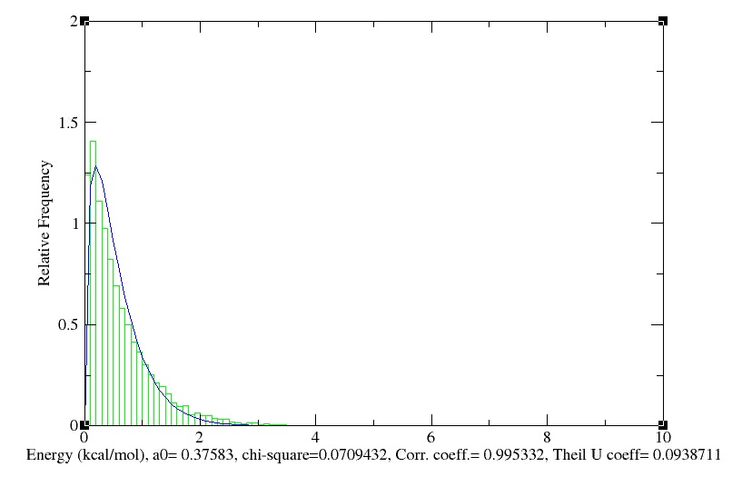
• Maxwell-Boltzmann Energy Distribution

We obtain the following histogramm!

• Temperature

Using EXCEL, we obtain the following graph, which represents the evolution of the temperature in function of time:

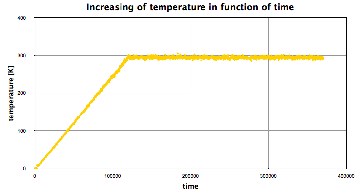
The first part corresponds the the heating, then we let the system reach an equilibrium (NPT state), a NVT portion, and finally a NPT portion again.

• Density

Using EXCEL, we obtain the following graph, which represents the evolution of the density in function of time:

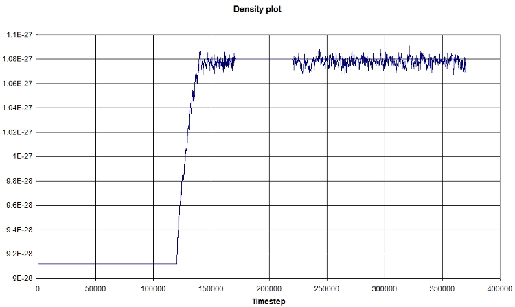
The first part corresponds the the heating, then we let the system reach an equilibrium (NPT state), a NVT portion, and finally a NPT portion again.

• Pressure

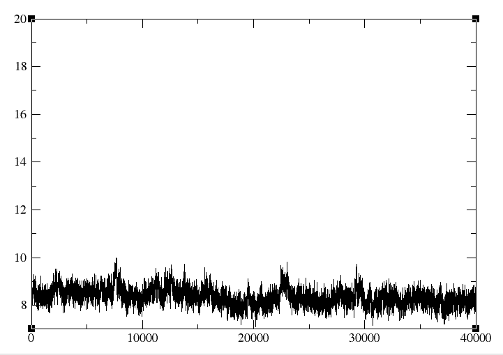
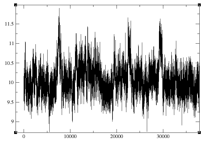
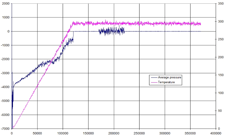
Here is a small plot of pressure and temperature in function of time

• RMSD

We obtain the following picture:

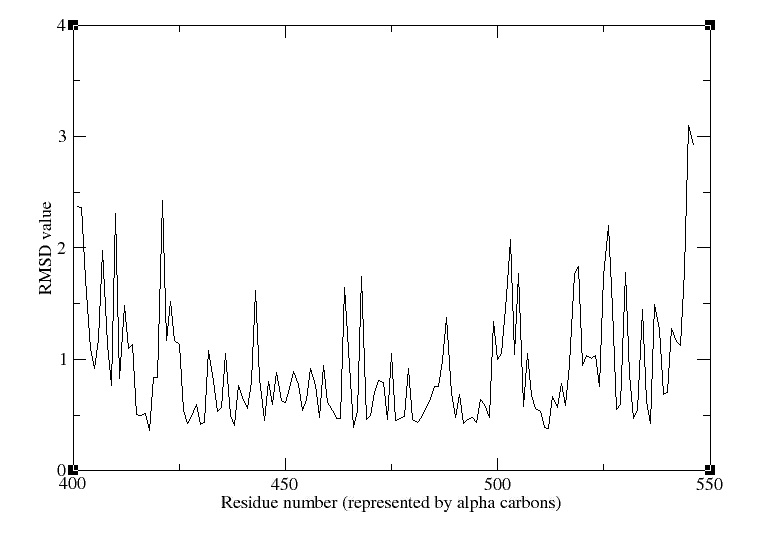
RMSD of residue within 3 angström of the FMN

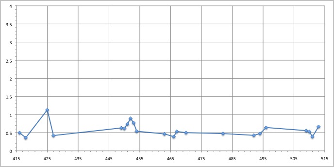
We can see that the residues that move the most are the residue number: 425, 451, 453

RMSD of residue within 6 angström of the FMN

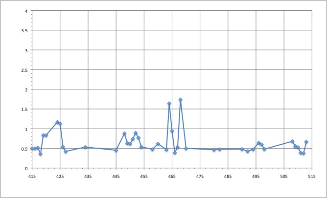
We can see that the residues that move the most are the residue number: 424, 425, 464, 468

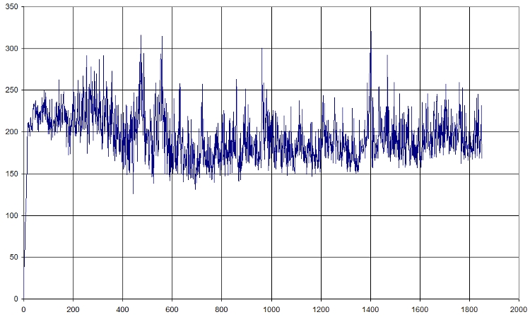
• RMSD of selected atoms compared to initial position along time

Here is a fast graph of the output of the average RMSD of the atoms in function of time. It seems normal.

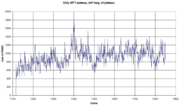
Here is what we got with FIRST_FRAME=1115 REFERENCE_FRAME=1115. Average=921.477, standard deviation=202.1708

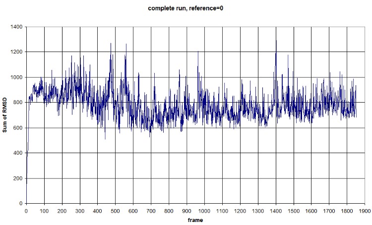
FIRST_FRAME=0 REFERENCE_FRAME=0. The difference of the sum probably comes from the new selection of atoms from the backbone. We should compute an average value to normalize amplitude. (fluctuation is conserved, anyway) Average=781.3913, standard deviation=118.1393

• Salt bridges

Here is a plot for one of the bridges. We have to look for the max distance for a salt bridge.

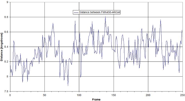
• RMSF

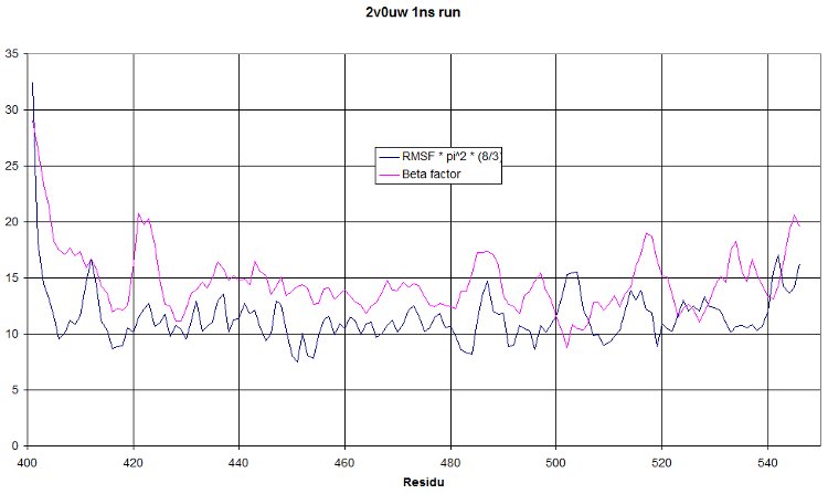
This is a 1 nanosecond NPT run at 300°K. We hope to see a RMSF curve identical to the beta factor. It should only be shifted higher because of the increased temperature. But having a similar tendency would mean our simulation show oscillations similar to what was observed during crystallography. This is really a quite nice validation of our run!

Differential analysis

Some useful distances

• Bond between Gln497 and Lys533 in light state

• Bond between Gln475 and Lys533 in light state