Team:EPF-Lausanne/Results/Validation

Temperature

Using EXCEL, we obtain the following graph, which represents the evolution of the temperature in function of time:

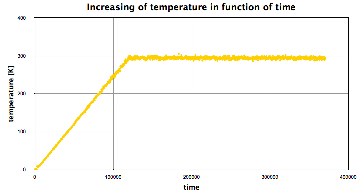
The first increasing part corresponds the the heating, then we let the system reach an equilibrium (NPT state), a NVT portion, and finally a NPT portion again. This is exactly what we wanted, and this prove we achieved to find a minimum in energy on the plateau.

Density

Using EXCEL, we obtain the following graph, which represents the evolution of the density in function of time:

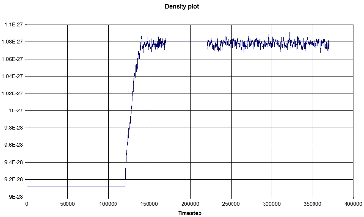
The first part corresponds the the heating, then we let the system reach an equilibrium (NPT state), a NVT portion, and finally a NPT portion again. The density plot follow the general scheme described above, and corroborate our findings.

Pressure

Here is a small plot of pressure and temperature in function of time
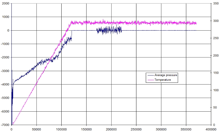
Again, it prove that we achieved our minimization, because the pressure following the increase in temperature, then during the NPT, the pressure remains constant (as stated!). The following portion is a NVT portion: this time, pressure is allowed to fluctuate to compensate other boundaries of volume and temperature. Finally, the last part is again a NPT part, and pressure is also constant.

RMSD

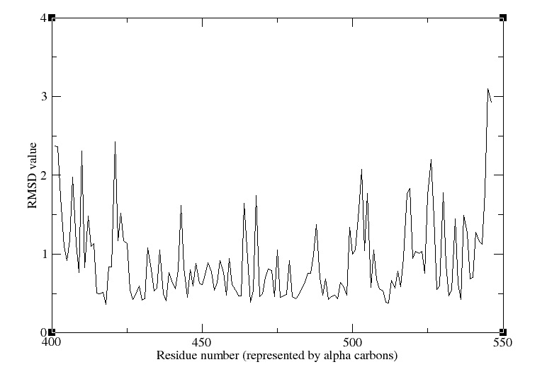
The root mean square deviation is a measure of the differences between predicted values and the values actually observed.
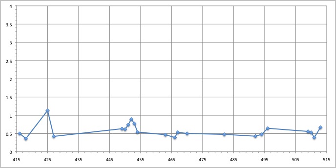
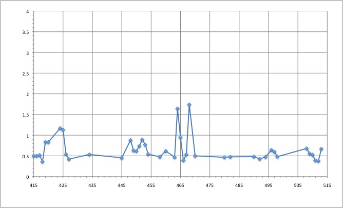
We obtain the following picture:

RMSD of residue within 3 angström of the FMN	RMSD of residue within 6 angström of the FMN
We can see that the residues that move the most are the residue number: 425, 451, 453	We can see that the residues that move the most are the residue number: 424, 425, 464, 468

RMSD of selected atoms compared to initial position along time

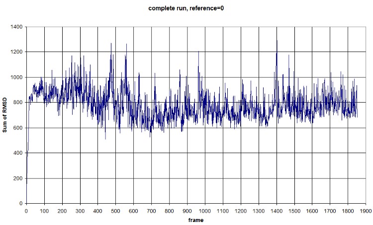
Here is a fast graph of the output of the average RMSD of the atoms in function of time. It seems normal.

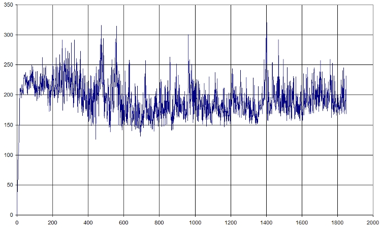
Here is what we got with FIRST_FRAME=1115 REFERENCE_FRAME=1115. Average=921.477, standard deviation=202.1708

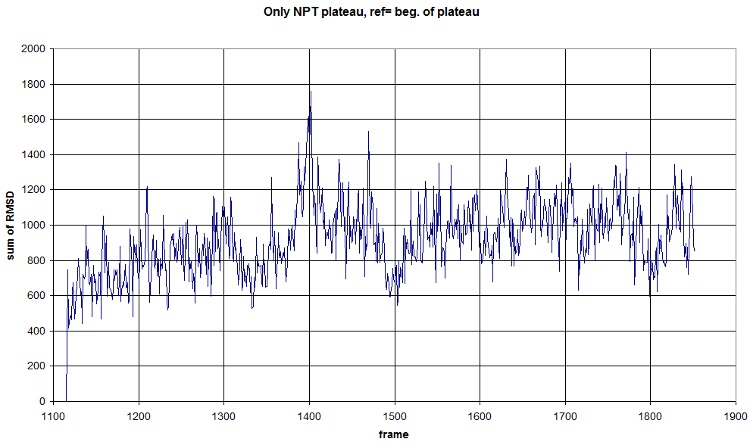
FIRST_FRAME=0 REFERENCE_FRAME=0. The difference of the sum probably comes from the new selection of atoms from the backbone. We should compute an average value to normalize amplitude. (fluctuation is conserved, anyway) Average=781.3913, standard deviation=118.1393

Salt bridges

They denotes a relatively weak ionic bond between positively charged amino acids (arginine or lysine) and negatively charged amino acids (asparatic acid or glutamic acid) in a protein. Salt bridges contribute to the stability of protein structure.
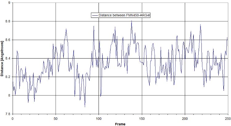
It has been hypothesized that activation arises as a result of the disruption of a salt bridge formed between two loops in the light state, but this remains speculation since the salt bridge is present in both light and dark state crystal structures (see Crosson, S., S. Rajagopal, and K. Moffat. 2003. The LOV domain family: photoresponsive signaling modules coupled to diverse output domains. Biochemistry. 42:2–10). However, we saw no significant difference in salt bridge behavior between the light and dark states, which is consistent with what found Freddolino, P.L., Dittrich M., Schulten K., Dynamic Switching Mechanisms in LOV1 and LOV2 Domains of Plant Phototropins.

Here is a plot for one of the bridges. We have to look for the max distance for a salt bridge.

RMSF

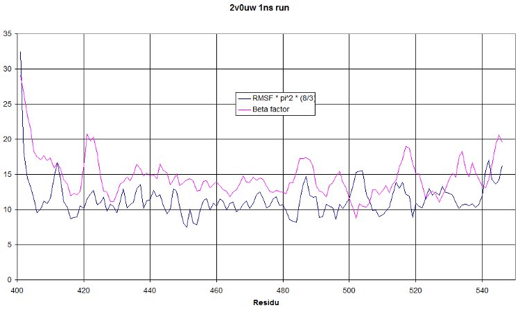
This is a 1 nanosecond NPT run at 300°K. We hope to see a RMSF curve identical to the beta factor. It should only be shifted higher because of the increased temperature. But having a similar tendency would mean our simulation show oscillations similar to what was observed during crystallography. This is really a quite nice validation of our run!