Team:Calgary/Modelling/Blog
From 2009.igem.org
UNIVERSITY OF CALGARY

|
September 3, 2009 - Afshin, Iman
MC Interface...Revealed!
Hi Everyone!
I am pleased to post (for the first time) screen shots of our Membrane Computing Agent Base Model. In this post i am focusing on interface mostly. Beside the fact that we want to have an accurate model, we also want a model that is easy to use. So we thought about design issues with our interface. How can we (computer scientists) hide as much code as possible so when a biologist uses our software, they don't freak out.
So lets take a look at our main screen: 
If the size of the picture is small and you have a hard time making out the details, you can always click on the photo and see a full size version. Unfortunately this is the largest size that the blog allows for posting images online. Anyways going back to our interface, on the top you see "Quorum Sensing Model - Version 2.0". So this is our QS model and the version 2.0 is our latest release. We initially started with version 1.0 and gone through 1.1, 1.2, 1.3, ... , 1.7. With versions 1.x we were adding basic functionality to the system. Simply setting up a framework, introducing rules, figuring out how to define rules and so on. In version 2.0 we have build the interface on top of our framework so users can interact with the system without the need of knowing how the code works. You don't need to compile anything, or type a single line of code. This is the beautify of Mathematica. I don't want to get into Mathematica and our implementation; however I want to mentioned that all you need to know to run our program is a shift+enter and that will do the trick. We have also worked on improving run-time speed of our simulation and I am happy to say that version 2.0 is about 5x faster than version 1.0! Going back to our interface, there are three different tabs on the top: Input, Visualization and About. Input tap includes 2 sub-tabs: Simulation parameters and Rule Constants. Under simulation parameters, we have different parameters to set before running the simulation. To get the user started, each parameter is set to a default value. User is able to modify each value before running the program. We will go over each parameter on our next post. For now lets focus on interface. We have different parameters for the simulation in general (population size and simulation step). Cytoplasm, Periplasmic space and environment also get their own list of parameters. At bottom of the interface we have a check box which allows user to introduce division into the mix. So there are two different way of running the simulation. When division check box is not selected, starting with 20 individual cells, the simulation ends with 20 cells and outputs a set of results. However when division checkbox is selected, user might start with 20 cells and based on how many steps is specified by the user, the system might end up with 40 or 80 cells. Results of the simulation also reflect the division. Next blow the checkbox we have a button for running the simulation and then the current status of simulation is shown below ("Ready!"). In order to give user an idea about current status of the simulation we have added a progress bar which only appears when the program is running. This progress bar gives the user a status update on how long will the simulation take before completion. Here is a screenshot of a simulation in progress: 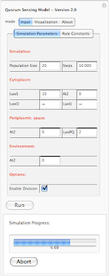
In this example the simulation is 69% completed. Next is looking at rule constants. Each rule in our simulation has a constant associated with it. This constant is used for calculating probability of a reaction. The system is loaded with default values for each constant. However one can modify each value before running the simualtion. Here is an screen shot of rule constants:  Because it is hard to remember which constant belongs to which rule, we have enabled a tool-tip option so when a user moves the mouse pointer over each constant, its corresponding interaction rule is displayed (as shown above). This should help out the user in associating each constant value with an interaction rule in the system. Because it is hard to remember which constant belongs to which rule, we have enabled a tool-tip option so when a user moves the mouse pointer over each constant, its corresponding interaction rule is displayed (as shown above). This should help out the user in associating each constant value with an interaction rule in the system. Here under about tab we plan to include copy rights, information about developers and other related information. There is also another aspect of our modeling project which is on hold for now due to time constraints. That is, ability of exporting results. Lets take a look at what we are planning to have maybe by end of this year:
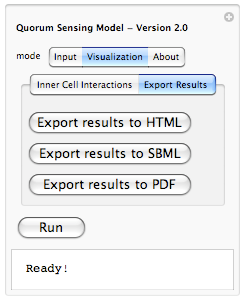 Yes, we are planning to integrate the ability of exporting results from the simulation to HTML (for posting online), SBML (Systems Biology Markup Language - for visualizing metabolic pathways and importing to popular biological modeling tools such as Cell Designer) and PDF (for sharing as well as printing). This is part of our future work for expanding the model and making it even more useful. Yes, we are planning to integrate the ability of exporting results from the simulation to HTML (for posting online), SBML (Systems Biology Markup Language - for visualizing metabolic pathways and importing to popular biological modeling tools such as Cell Designer) and PDF (for sharing as well as printing). This is part of our future work for expanding the model and making it even more useful.If you have been wondering about results, well our model is also able to produce nice and clean graph visualizations. Lets take a look at sample AI2 concentration over 1000 steps:
 I am gong to present only this graph for our result section just to demonstrate that our model is able to not only simulate by also analyze the results and visualize them. Ok. This should do it for now. Consider this post as a sneak preview of what hopefully will be a complete Quorum Sensing Model. We hope to have our completed model posted on UCalgary wiki by end of september. Thanks for following our progress! Afshin
|
|
August 17, 2009 - Carol, Chinee, Kevin, Vicki
Sensitivity analysis... Models... Have feelings too!
Vicki and Chinee have put quite an amout of time into tracking down those sensitive ones in our system. Vicki is currently working with the Sensitivity analysis tool in Matlab commandline in order to find the sensitive parameters that influence the GFP output the most. The following graph is the result her sensitivity analysis model has generated so far: (click to enlarge)
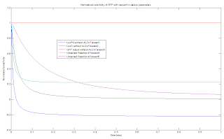
The closer the graph gets to 0, the lower the influence this parameter has on the GFP output, and vice versa. According to this graph, the kForward (reaction rates)values 1, 3, and 4 seems the most influential parameters relative to 2 and 5; thus these parameters will be looked at further. From these results, Vicki performed parameter optimization on them. In parameter optimization function, she was able to play with the individual parameter values in order to come up with a best fit line model to the predicted levels of GFP output. The following is the graphical result of the above function. 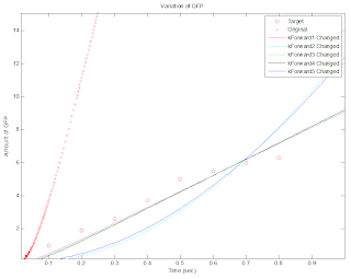
Here, the circles represent the made up predicted data, and the colored lines represent each optimized parameters. The optimized rate constants for kForward1, 3, and 4 fit nicely to the pattern of the predicted data; however, the optimized rate constants for kForward 2 and 5 do not, meaning that these parameters do not play a big role in determining the GFP output values. From these two functions, Vicki would be able to, once we get some lab results, optimize our significant rate constants to fit the behavior of our AI-2 system. Along with Vicki, Chinee was also working on the parameter sensitivity; however, with a different tool. In Simbiology, Chinee was able to outline the key difference between the initial amount and the reaction rates of the parameter. The following is the graph when all the parameters have a reaction rate value of 1: 
The following is the graph when all the parameters have a reaction rate value of 10: 
The only difference between the above two graphs are that the lines in the second graph are much more steep than the lines in the first graph. This means that the reaction rate only influences how immediate the reactions happen. And finally, the graph when all the parameters have an initial amount of 10: 
The above graph is very different from the ones above. From this, one can see how initial amounts of parameter play a much bigger role than the rate constants of each parameters. I, Kevin, and Carol attempted to fix some biological misunderstandings within the reactions, and produce a graph that displays the pattern of each parameters. The following is the graph: 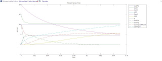
The patterns observed are reasonable and match what was expected. The lab data is needed to get an accurate model of our system; however, from it we can still test the sensitivity of each parameters by changing them one by one and simulating the results. We hope to get some lab data by this week. |
|
August 8, 2009 - Afshin & Iman
Membrane Computing Update
Hi Everyone!
This will be our first update on Membrane Computing (MC) and agent-based approach to model our complex biological system. In regards to modeling of Autoinducer-II Quorum Signaling, we have been able to successfully complete our implementation of this signaling cascade. Monitoring each cell as an agent, we are able to monitor the system at both, cell level and population level. Currently our simulation uses a well known algorithm called Gillespie's Algorithm. In simple words, the Gillespie algorithm keeps stochasticity (randomness) in our simulation. Why is it important to have this randomness in our model? Because this will push our model one step closer to actual biological system. Because cells don't interact with each other or their environment at discrete steps. As an example consider protein-protein interactions versus cell division. These two interactions have quite different time scales. Our implementation of Gillespie Algorithm takes care of accounting for such cases. At this stage our model is able to produce concentration graphs and allows user to review how the system behaves at the cell level and also at colony level. We are working on implementing powerful visualizations and a user-friendly interface for our model. We are also working on addition of new updating scheme for cells during simulation. Currently our algorithm updates state of each cell at single steps. It is worth mentioning that because of the way our Gillespie Algorithm is setup, time delays between each step can be as short as 0.0001 second (considered instantaneous) or a given step could take as long as one minute. This will compensate for different interactions and the time it takes for each interaction to complete. The second scheme which we are working now to complete hopefully before aGEM is where all cells in the system are updated at the same time. This allows cells to be in sync when applying interactions. With single-step updating scheme, as the number of cells increase over time, it takes longer and longer for cells to update their state based on changes in their environment. This side effect of non-synchronous updating scheme only kicks in when we have high population of cells. Since we have introduced cell division to our simulation where our system could start with one cell and end up with 300, a synchronous updating system could take us one step closer to how the actual biological system works. We will post updates at least once a week on our current progress; We also hope to have some screen shots on our visualizations and interface in near future. Thanks for following our progress :) |
|
August 3, 2009 - Carol
Modelling: Collaborative Work
Hi Everyone! Not much to update for modelling this week. We had a big meeting with all the teams on friday, and the two modelling teams (Membrane Computing and Mathematical Modelling) will meet every tuesday and thursday for meetings. This will give us time to draw parallel between the two types of modelling. We have also discussed about how to seperate all the experiments to characterize our signalling system. All this detail will be touched tomorrow at the meeting. Other than that, not much to update. Hopefully next week, we have more to add! Peace :)
|
|
July 27, 2009 - Carol
Modelling: Learning to Write
Hi everyone, its Carol again!
This week for modeling, we focused mainly on writing up several ways to characterize the AI-2 signaling system. The characterization methods that we decided to explore are the following: 1. Static Performance 2. Dynamic Response 3. Response Time 4. Robustness The robustness part of characterizing the system would be the most interesting. The degree of robustness depends on how sensitive the system is to fluctuations and changes. If this part of the signaling system can be explored in more detail, it will be an advantageous component to our project. We spent the past week summarizing this in paper format. I am currently working on a promoter library, which will play a huge role in exploring the expression of luxPQ. Once the circuits are done, some of these experiments can be done in a few days. We will hopefully by the end this summer have some characterization done. Stay tuned! Signing off now, peace! |
|
July 21, 2009 - Vicki
iGEM's Next Top Model?
Hey there! So I’m a little late with this entry…hopefully none of you are too crushed by this. As a refresher, I’m Vicki, and we’ve already met repeatedly over lab editions. With my fabulous team of brilliance – Carol, Chinee, Kevin, Afshin and Iman – we’re going to give the term “America’s next top model” a whole new meaning.
It has been a very busy week of searching for reaction constants for our differential and membrane-computing efforts. Indeed, the literature is vast, but it sure isn’t easy to navigate. And it doesn’t help when published authors don’t really seem to make effective communication a priority. Regardless, we’re progressing, slowly but surely. We have also been discussing how we’re going to approach the circuit characterisation matter. After a long and fruitful chat on what others have done previously to characterise their signalling circuits, we came up with a list of areas for which quantitative characterisation would be useful AND realistic to achieve. Because as much as we want to pay for sequencing every day to assess circuit stability, it doesn’t seem like the most effective use of our funds, especially with so other areas (read: ice cream parties) where the money would be better spent! We also outlined general procedure approaches that would enable us to collect the data to come up with and validate our models. Stay tuned! |
|
July 13, 2009 - Kevin
Techy Biologist
|
|
July 6, 2009 - Carol
Modelling: How Engineers Understand the Social Life of Bacteria
Hi! My name is Carol and I’m heading into my third year of biomedical and chemical engineering in the fall, and I have completed a degree in biomedical sciences. I love watching sports (especially football and hockey) and I enjoy cooking and reading. I’m part of the laboratory and modelling team, so you’ll be hearing from me lots this summer!
In the past few weeks, the modelling team focused on familiarizing with Matlab and Simbiology. Before I move on, I should introduce you to my team mates that make this team possible! Vicki is a recent graduate from Engineering from the University of Toronto and she has worked with Matlab and its applications extensively throughout her studies. Chinee is also a third year chemical engineering and has some experience with Matlab as well. Finally, Kevin who is going into his second year of Kinesiology is just helping out because he is just a nice individual! With all the skills from each team member, we believe that we can produce a great model for our project. Back to modelling, one of our facilitators (Dr. Nygren) gave us an assignment that helped us understand the program more. We had to model the three gene repressilator in Matlab via two different methods, stochastic and deterministic. I’m going to spend some time now to explain the two methods that we will be using to model our quorum sensing model. Differential (Deterministic) Model This model uses equations that involve derivatives to illustrate concentrations of different molecules within a network. In our case, we will be using equations to describe the concentrations of different molecules within the Autoinducer-II (AI-2) cascade. With the ability to solve the differential equations, we can investigate how the concentration of different molecules within the cascade modifies compared with initial conditions. However, this method of modelling is often used with systems with high concentrations of chemicals and we expect that the importance of rare events is low. Furthermore, this type of modelling is often used in smaller networks. Stochastic Models The other type of model that can be used to describe our model is through probabilistic equations that can describe the probability that a certain chemical reaction will occur between certain types of molecules at any instant. Furthermore, these equations can also be used to calculate the quantities of all species at the end of a small time step. Therefore, it is plausible to evaluate how the molecules within the cascade change over time by repeating this process over many steps. Since random variable input is involved with this type of modelling, each simulation run can produce varying results. By using averages through numerous simulation runs, a trend can be predicted. This type of modelling is used for small numbers of molecules because they take more computing power. This is because of the random nature of molecular interaction and it accounts for the probability of rare events occurring. Our goal for this week is to successfully build the AI-2 system in Simbiology. We’ve been busy the last few weeks reading up on literature and we were able to successfully find some phosphorylation rates that can be incorporated into our model. Next week, we will show you what we’ve built in Simbiology and give you a tour of Simbiology and Matlab! Stay Tuned! |
 "
"


