Team:SJTU-BioX-Shanghai/Modelling
From 2009.igem.org
Pnstontale (Talk | contribs) m |
Pnstontale (Talk | contribs) m |
||
| (29 intermediate revisions not shown) | |||
| Line 5: | Line 5: | ||
==Motivation== | ==Motivation== | ||
| - | From the | + | From the introduction of our system, one can see that our model is designed to regulate the bio-clock of '''''E.coli'''''. However, this system is more complicated than one can think in that it consists of a variety of reactions, which is quite hard for us to analysis without mathematics. So it is indispensible to justify that the concentration of relE will oscillate with a specific periodicity. Moreover, understanding the important parameters of the system allows one to choose appropriate promoters and rbses to make our system work. Therefore, we have created the mathematical models to prove our project is feasible, to guide our experiment, and to predict the length of '''''E.coli'''''’s sleeping time. |
| - | + | ||
==Introduction== | ==Introduction== | ||
| - | First of all, let's pick out the three key genes, which | + | First of all, let's pick out the three key genes, which are named '''''relE''''', '''''relB''''' and '''''Lon''''', from the original network. Then the interaction between them can be expressed in the following picture. |
| - | [[Image: | + | [[Image:SJTU09_Modeling_html5.jpg|center|thumb|580px|Interaction between '''''relE''''', '''''relB''''' and '''''Lon''''']] |
| - | Actually, there are four types of reactions in | + | Actually, there are four types of reactions in our system, which are highlighted with different colors. |
| - | * The arrow marked | + | * The arrow marked in green represents a single gene expression |
| - | * The arrow marked | + | * The arrow marked in yellow represents relE cleavage process |
| - | * The arrow marked | + | * The arrow marked in blue represents relB-Lon hydrolysis |
| - | * the arrow marked | + | * the arrow marked in purple represents relE and relB polymerization |
| - | + | ||
| - | + | ||
| + | From the picture mentioned above, obviously almost every two genes or its mRNAs have a bio-chemical reaction. | ||
==Assumptions and hypothesis == | ==Assumptions and hypothesis == | ||
| - | # The number of | + | # The number of ribosomes in '''''E.coli''''' is sufficiently large at all times |
| - | # The cleavage reaction caused by relE is | + | # The cleavage reaction caused by relE is an enzyme process |
| - | # Any protein | + | # Any protein or its related mRNA generates at a constant rate |
# Either protein or mRNA degrades in direct ratio to its concentration | # Either protein or mRNA degrades in direct ratio to its concentration | ||
| - | In order to make | + | In order to make a quantitative analysis, we should simplify our model by making the above-mentioned assumptions. The first one is the vital assumption in our system. Since a cell may have thousands of ribosomes and the number is positively correlated with growth rate<sup><nowiki>[1]</nowiki></sup>, we consider this assumption reasonable. In fact we can overlook the other side of this assumption, which will lead us to deal with the piecewise ODEs (ordinary differential equations).Unfortunately, such kind of equations can hardly be solved by Matlab. The second assumption is supported by ''The Bacterial Toxin RelE Displays Codon-Specific Cleavage of mRNAs in the Ribosomal A Site''<sup><nowiki>[2] </nowiki></sup>while the last two assumptions are illustrated by ''Stochastic simulations Application to molecular networks''<sup><nowiki>[3]</nowiki></sup>. |
| - | + | ||
==Model development == | ==Model development == | ||
| Line 38: | Line 35: | ||
===Single gene expression=== | ===Single gene expression=== | ||
| - | According to assumption 3 and 4 | + | According to assumption 3 and 4 we have made, we deduce the following six equations: |
[[Image:SJTU09 Modeling html1.gif|center]] | [[Image:SJTU09 Modeling html1.gif|center]] | ||
| - | Where '''''α<sub>1</sub>''''', '''''α<sub>3</sub>'''''and '''''α<sub>5</sub>''''' represent the strength of promoters. '''''α<sub>2</sub>''''', '''''α<sub>4</sub>''''' and '''''α<sub>6</sub>'''''represent the strength of rbs. '''''β<sub>i</sub>(i=1,2...6)''''' | + | Where '''''α<sub>1</sub>''''', '''''α<sub>3</sub>'''''and '''''α<sub>5</sub>''''' represent the strength of promoters. '''''α<sub>2</sub>''''', '''''α<sub>4</sub>''''' and '''''α<sub>6</sub>'''''represent the strength of rbs. '''''β<sub>i</sub>(i=1,2...6)''''' represents the degradation rate of the associated proteins or mRNAs. |
| - | + | ||
===relE cleavage process=== | ===relE cleavage process=== | ||
| Line 56: | Line 52: | ||
===relB-Lon hydrolysis=== | ===relB-Lon hydrolysis=== | ||
| - | For relB-Lon hydrolysis, we | + | For relB-Lon hydrolysis, we also regard it as Michaelis-Menten equation: |
[[Image:SJTU09 Modeling html3.gif|center]] | [[Image:SJTU09 Modeling html3.gif|center]] | ||
| - | Where '''''k<sub>m</sub>''''' is | + | Where '''''k<sub>m</sub>''''' is Michaelis constant, which is related with the affinity of the Lon. '''''k<sub>cat0</sub>''''' is related with both relB and Lon. |
| - | + | ||
===relE and relB polymerization=== | ===relE and relB polymerization=== | ||
| - | For relE and relB polymerization, we | + | For relE and relB polymerization, we considered it as the second-order reaction: |
[[Image:SJTU09 Modeling html4.gif|center]] | [[Image:SJTU09 Modeling html4.gif|center]] | ||
where k represents the reaction coefficient. | where k represents the reaction coefficient. | ||
| - | |||
===Modeling the full system=== | ===Modeling the full system=== | ||
| Line 114: | Line 108: | ||
*h: Lon degradation rate | *h: Lon degradation rate | ||
| - | Now, we are ready to calculate the right value of these eight parameters by Matlab. Remember our target is to select the proper parameters to make the system oscillate. If so, the bacteria will fall asleep when relE rises to a high level | + | Now, we are ready to calculate the right value of these eight parameters by Matlab. Remember our target is to select the proper parameters to make the system oscillate. If so, the bacteria will fall asleep when relE rises to a high level while it will be active when relE falls down to a low level. |
We set the following value for the parameters, to see if they satisfy our requirement. | We set the following value for the parameters, to see if they satisfy our requirement. | ||
| Line 125: | Line 119: | ||
At first we find that the majority of the systems with specific parameters are asymptotic stable. In order to figure out the reason why they cannot show us oscillations, we consider the oscillation criterion. | At first we find that the majority of the systems with specific parameters are asymptotic stable. In order to figure out the reason why they cannot show us oscillations, we consider the oscillation criterion. | ||
| - | <center><font size=4>[[judge_a_system|'''How to judge a system that cannot oscillate?''']]</font></center> | + | <center><font size=4>[[Team:SJTU-BioX-Shanghai/judge_a_system|'''How to judge a system that cannot oscillate?''']]</font></center> |
| - | With the help of the criterion, we can remove many situations which will lead to asymptotic stable. This will reduce the burden of matlab to some degree. Matlab tells us the following | + | With the help of the criterion, we can remove many situations first which will lead to asymptotic stable. This will reduce the burden of matlab to some degree. Matlab tells us the following parameters' value can help the system reach an oscillation state. |
[[Image:SJTU09 Modeling html9.gif|center]] | [[Image:SJTU09 Modeling html9.gif|center]] | ||
| - | And these parameter value listed below will lead to a | + | And these parameter value listed below will lead to a damped oscillation state. |
[[Image:SJTU09 Modeling html10.gif|center]] | [[Image:SJTU09 Modeling html10.gif|center]] | ||
| - | After | + | After several minutes work by Matlab, one can see the following three situations with specific parameter values. |
===oscillate with periodicity=== | ===oscillate with periodicity=== | ||
| - | [[Image:SJTU09_Modeling_html1.jpg|center|thumb| | + | [[Image:SJTU09_Modeling_html1.jpg|center|thumb|590px|oscillate with periodicity]] |
===damped oscillations=== | ===damped oscillations=== | ||
| - | [[Image:SJTU09_Modeling_html2.jpg|center|thumb| | + | [[Image:SJTU09_Modeling_html2.jpg|center|thumb|590px|damped oscillations]] |
===equilibrium states=== | ===equilibrium states=== | ||
| - | [[Image:SJTU09_Modeling_html3.jpg|center|thumb| | + | [[Image:SJTU09_Modeling_html3.jpg|center|thumb|590px|equilibrium states]] |
| - | + | ||
==Conclusion== | ==Conclusion== | ||
| Line 155: | Line 148: | ||
[[Image:SJTU09_Modeling_html11.gif|center]] | [[Image:SJTU09_Modeling_html11.gif|center]] | ||
| - | From these pictures, it is obvious that a larger value of “a” means a higher probability of oscillation. In addition, a less value of “d” means a higher probability of oscillation. Moreover, the value of “g” plays an important role in oscillation system. We find that when we set the value of “g” lower than 13, then this system | + | From these pictures, it is obvious that a larger value of “a” means a higher probability of oscillation. In addition, a less value of “d” means a higher probability of oscillation. Moreover, the value of “g” plays an important role in oscillation system. We find that when we set the value of “g” lower than 13, then this system falls into chaos. When we set the value of “g” from 18 to 22, we observe the oscillations. When we set the value of “g” higher than 25, the system reduces to damping oscillations and reach the equilibrium state immediately. In conclusion, we can set g=22 to have the best effect. According to our former discussion, we are now able to choose the appropriate promoters to make our system oscillate. |
| - | + | ==References & Attachment== | |
| - | ==References & | + | |
<nowiki>[1]</nowiki> Michael T. Madigan, John M. Martinko, ''Brock biology of microorganism 11th edition, ''Pearson Education International 2006, ISBN:0-13-196893-9 | <nowiki>[1]</nowiki> Michael T. Madigan, John M. Martinko, ''Brock biology of microorganism 11th edition, ''Pearson Education International 2006, ISBN:0-13-196893-9 | ||
| Line 170: | Line 162: | ||
| - | Since this site doesn't support Tex format for formulas, we provide our<br />source document [ | + | Since this site doesn't support Tex format for formulas, we provide our<br />source document [https://static.igem.org/mediawiki/2009/9/99/SJTU09_Modeling.zip SJTU09 Modeling.zip] for you to download. |
| + | |||
| + | Go to see [[Team:SJTU-BioX-Shanghai/Protocols#bannerTop|Protocols]]. | ||
{{Template:SJTU09_enddiv}} | {{Template:SJTU09_enddiv}} | ||
Latest revision as of 07:44, 21 October 2009

Project introduction. Inspired by the natural regulator of circadian bioclock exhibited in most eukaryotic organisms, our team has designed an E.coli-based genetic network with the toxin-antitoxin system so that the bacterium oscillates between two states of dormancy and activity (more...)
Contents[hide] |
Motivation
From the introduction of our system, one can see that our model is designed to regulate the bio-clock of E.coli. However, this system is more complicated than one can think in that it consists of a variety of reactions, which is quite hard for us to analysis without mathematics. So it is indispensible to justify that the concentration of relE will oscillate with a specific periodicity. Moreover, understanding the important parameters of the system allows one to choose appropriate promoters and rbses to make our system work. Therefore, we have created the mathematical models to prove our project is feasible, to guide our experiment, and to predict the length of E.coli’s sleeping time.
Introduction
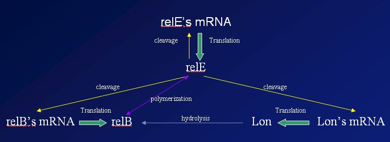
First of all, let's pick out the three key genes, which are named relE, relB and Lon, from the original network. Then the interaction between them can be expressed in the following picture.
Actually, there are four types of reactions in our system, which are highlighted with different colors.
- The arrow marked in green represents a single gene expression
- The arrow marked in yellow represents relE cleavage process
- The arrow marked in blue represents relB-Lon hydrolysis
- the arrow marked in purple represents relE and relB polymerization
From the picture mentioned above, obviously almost every two genes or its mRNAs have a bio-chemical reaction.
Assumptions and hypothesis
- The number of ribosomes in E.coli is sufficiently large at all times
- The cleavage reaction caused by relE is an enzyme process
- Any protein or its related mRNA generates at a constant rate
- Either protein or mRNA degrades in direct ratio to its concentration
In order to make a quantitative analysis, we should simplify our model by making the above-mentioned assumptions. The first one is the vital assumption in our system. Since a cell may have thousands of ribosomes and the number is positively correlated with growth rate[1], we consider this assumption reasonable. In fact we can overlook the other side of this assumption, which will lead us to deal with the piecewise ODEs (ordinary differential equations).Unfortunately, such kind of equations can hardly be solved by Matlab. The second assumption is supported by The Bacterial Toxin RelE Displays Codon-Specific Cleavage of mRNAs in the Ribosomal A Site[2] while the last two assumptions are illustrated by Stochastic simulations Application to molecular networks[3].
Model development
Single gene expression
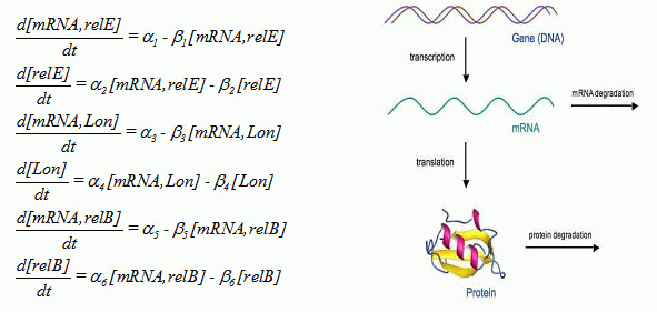
According to assumption 3 and 4 we have made, we deduce the following six equations:
Where α1, α3and α5 represent the strength of promoters. α2, α4 and α6represent the strength of rbs. βi(i=1,2...6) represents the degradation rate of the associated proteins or mRNAs.
relE cleavage process
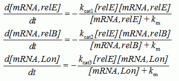
Based on assumption 1 and 2, we choose the classical Michaelis-Menten equations to describe the relE cleavage process:
Where km is the Michaelis constant, which is only related with the affinity of the enzyme (relE) for the substrate. kcati(i=1,2,3) is related with the cleavage rate of relE.
relB-Lon hydrolysis
For relB-Lon hydrolysis, we also regard it as Michaelis-Menten equation:
Where km is Michaelis constant, which is related with the affinity of the Lon. kcat0 is related with both relB and Lon.
relE and relB polymerization
For relE and relB polymerization, we considered it as the second-order reaction:
where k represents the reaction coefficient.
Modeling the full system
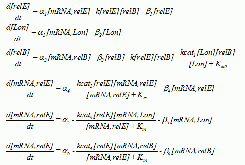
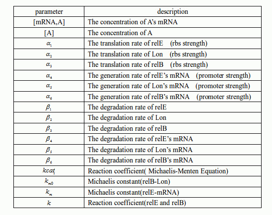
Based on the former analysis, we can generalize our model into the following six ordinary differential equations:
The following table shows the description of the parameters.
However, since we proposed these equations, we began to realize some problems for us before we can get satisfactory results from them:
- From the table above, we can see that there are heaps of parameters for us to find out. And some of them are even impossible for us to get.
- We are only interested in the amounts of some proteins, mainly the relB and relE. However, there are many other things, such as the various mRNA, for us to cope within the equations.
- The complexity of the relations among different elements adds great difficulties for us to calculate and analyze.
So, we decided to only focus on the relations between two of the three proteins, which mostly interests us.
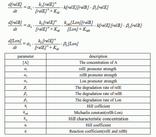
Having the above notion in our minds, we proposed our simplified new model. We keep the majority of the terms in our new model, except the relE cleavage term. Since we are not pretty sure about the principle of relE cleavage process, we choose the classical hill equations. Now, we can write down our new model in the following three ordinary differential equations:
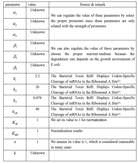
Now, we can see the new model is much simpler for Matlab to cope with. However, we still should find the values of some parameters from a variety of databases. They are listed as below:
Since most parameters can be found in several papers, what we should do is to choose the appropriate parameters, such as the promoter strength and the degradation rate, to make the system oscillate. Fortunately, Matlab can handle all these works, which will be presented in the next section.
Simulation
At the beginning of the simulation part, let's replace the parameters with simple characters.
- a: relE promoter strength
- b: relE degradation rate
- c: Reaction coefficient(relE and relB)
- d: relB promoter strength
- e: relB degradation rate
- f: reaction coefficient(Lon and relB)
- g: Lon promoter strength
- h: Lon degradation rate
Now, we are ready to calculate the right value of these eight parameters by Matlab. Remember our target is to select the proper parameters to make the system oscillate. If so, the bacteria will fall asleep when relE rises to a high level while it will be active when relE falls down to a low level.
We set the following value for the parameters, to see if they satisfy our requirement.
a = {11,16,21,26,31};b = {1,6};c = {1,6,11};d = {21,26,31};
e = {1,6};f = 46;g = {21,26,31};h = {1,6}
At first we find that the majority of the systems with specific parameters are asymptotic stable. In order to figure out the reason why they cannot show us oscillations, we consider the oscillation criterion.
With the help of the criterion, we can remove many situations first which will lead to asymptotic stable. This will reduce the burden of matlab to some degree. Matlab tells us the following parameters' value can help the system reach an oscillation state.
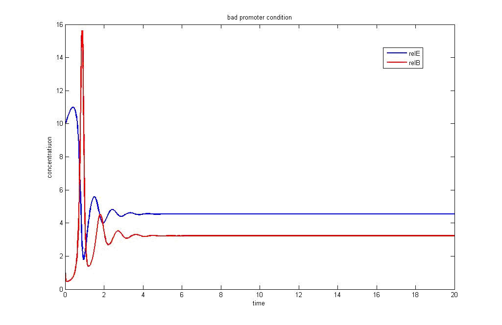
And these parameter value listed below will lead to a damped oscillation state.
After several minutes work by Matlab, one can see the following three situations with specific parameter values.
oscillate with periodicity
damped oscillations
equilibrium states
Conclusion
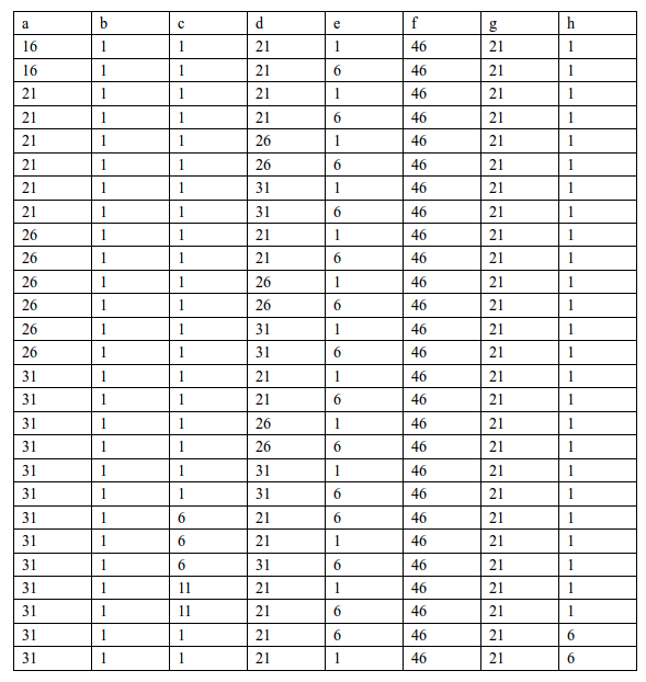
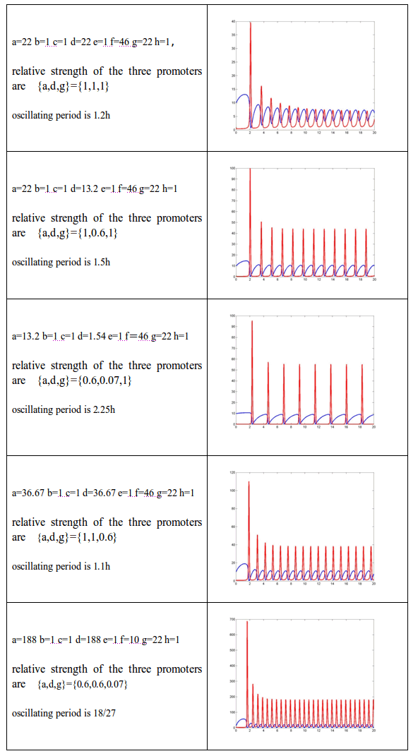
Since we have three types of promoters (j23110,j23118,j23116) with their relative strength 1:0.6:0.07, we are now able to choose the proper one to make our system oscillate. All the well-performing situation are listed as below:
From these pictures, it is obvious that a larger value of “a” means a higher probability of oscillation. In addition, a less value of “d” means a higher probability of oscillation. Moreover, the value of “g” plays an important role in oscillation system. We find that when we set the value of “g” lower than 13, then this system falls into chaos. When we set the value of “g” from 18 to 22, we observe the oscillations. When we set the value of “g” higher than 25, the system reduces to damping oscillations and reach the equilibrium state immediately. In conclusion, we can set g=22 to have the best effect. According to our former discussion, we are now able to choose the appropriate promoters to make our system oscillate.
References & Attachment
[1] Michael T. Madigan, John M. Martinko, Brock biology of microorganism 11th edition, Pearson Education International 2006, ISBN:0-13-196893-9
[2] Kim Pedersen, Andrey V. Zavialov,Michael Yu. Pavlov, Johan Elf,Kenn Gerdes, and Mans Ehrenberg. The Bacterial Toxin RelE Displays Codon-Specific Cleavage of mRNAs in the Ribosomal A Site. Cell, Vol. 112, 131–140, January 10, 2003
[3] Didier Gonze, Stochastic simulations Application to molecular networks March 27, 2007
Since this site doesn't support Tex format for formulas, we provide our
source document SJTU09 Modeling.zip for you to download.
Go to see Protocols.
 "
"
