Team:Groningen/Modelling/Characterization
From 2009.igem.org
(Some tweaks to our characterization page.) |
m (→{{anchor|Optimization}}Optimization procedure) |
||
| (8 intermediate revisions not shown) | |||
| Line 1: | Line 1: | ||
{{Team:Groningen/Modelling/Header}} | {{Team:Groningen/Modelling/Header}} | ||
| + | <div style="float:left" >{{linkedImage|GroningenPrevious.png|Team:Groningen/Modelling/Arsenic}}</div> | ||
| + | |||
<div title="Arsie Says UP TO ACCUMULATION" style="float:right" >{{linkedImage|Next.JPG|Team:Groningen/Modelling/Downloads}}</div> | <div title="Arsie Says UP TO ACCUMULATION" style="float:right" >{{linkedImage|Next.JPG|Team:Groningen/Modelling/Downloads}}</div> | ||
| + | <div style="clear:both;"></div> | ||
| + | |||
| + | <html><style type="text/css"> | ||
| + | .intro { margin-left:0px; margin-top:10px; padding:10px; border-left:solid 5px #FFF6D5; border-right:solid 5px #FFF6D5; text-align:justify;background:#FFFFE5; } | ||
| + | </style></html> | ||
<div class="intro introduction"> | <div class="intro introduction"> | ||
==Characterization== | ==Characterization== | ||
We have four kinds of parts we would like to characterize: Importers, Accumulators, Sensors and the GVP cluster. | We have four kinds of parts we would like to characterize: Importers, Accumulators, Sensors and the GVP cluster. | ||
| - | For this we have a number of methods to estimate | + | For this we have a number of methods to estimate ''specific parameters'' (detailed below), as well as a ''[[Team:Groningen/Modelling/Characterization#Optimization|stochastic tool to fit our model]]'' to experimental data based on simulated annealing. |
</div> | </div> | ||
| Line 151: | Line 158: | ||
=={{anchor|Optimization}}Optimization procedure== | =={{anchor|Optimization}}Optimization procedure== | ||
| - | To fit our model to experimental data from different uptake experiments and/or papers we have implemented an optimization procedure that allows for experiments with different genotypes and circumstances by letting constants be overridden per experiment. It aims to optimize the sum of the RMS errors for each experiment using Simulated Annealing. By clicking the button "Fit" the optimization is started and its progress can be followed by looking at the table of constants and the graphs shown below the table (which are updated in real-time as the best solution is improved). | + | To fit our model to experimental data from different uptake experiments and/or papers we have implemented an optimization procedure that allows for experiments with different genotypes and circumstances by letting constants be overridden per experiment. It aims to optimize the sum of the RMS errors for each experiment using Simulated Annealing. By clicking the button "Fit" the optimization is started and its progress can be followed by looking at the table of constants and the graphs shown below the table (which are updated in real-time as the best solution is improved). In the optimizations procedure the ratio between v5 and K5 is kept constant. This is done because this ratio could be determined exactly using the data from the experiments done by [[Team:Groningen/Literature#Meng2004|Meng 2004]] v5 itself is not fixed and may vary. (Note that in the code different experiments and graphs can be enabled/disabled, we have entered data from Kostal, Meng and our first ICP-MS measurements.) |
{| | {| | ||
| Line 261: | Line 268: | ||
|id="betaKcurgradient"| | |id="betaKcurgradient"| | ||
|id="betaKsol"| | |id="betaKsol"| | ||
| - | + | |- | |
|tauGbeta5 | |tauGbeta5 | ||
|id="tauGbeta5"| | |id="tauGbeta5"| | ||
| Line 278: | Line 285: | ||
|id="beta5cur"| | |id="beta5cur"| | ||
|id="beta5curgradient"| | |id="beta5curgradient"| | ||
| - | |id="beta5sol"| | + | |id="beta5sol"| |
|- | |- | ||
|ars2T | |ars2T | ||
| Line 309: | Line 316: | ||
time:[1.127*60,4.993*60,9.986*60,20.159*60,30.181*60,60.035*60]}}, | time:[1.127*60,4.993*60,9.986*60,20.159*60,30.181*60,60.035*60]}}, | ||
Kostal2004fig3A: // fig 3A | Kostal2004fig3A: // fig 3A | ||
| - | {constants:{Vc:0.006666667,Vs:(1-0.006666667),pro:0,ars2T:0,proK:1.6605e-9},time: | + | {constants:{Vc:0.006666667,Vs:(1-0.006666667),pro:0,ars2T:0,proK:1.6605e-9},time:3600, |
data:{AsinT:[28.71e-6,78.87e-6,144.21e-6,377.19e-6,490.38e-6,617.76e-6,649.11e-6], | data:{AsinT:[28.71e-6,78.87e-6,144.21e-6,377.19e-6,490.38e-6,617.76e-6,649.11e-6], | ||
AsT:[0.4e-6,1e-6,2e-6,5e-6,20e-6,50e-6,100e-6]}}, | AsT:[0.4e-6,1e-6,2e-6,5e-6,20e-6,50e-6,100e-6]}}, | ||
| Line 326: | Line 333: | ||
pArsRRFPcon: // here the cell only contains extra RFP behind the the extra ArsR promoters. | pArsRRFPcon: // here the cell only contains extra RFP behind the the extra ArsR promoters. | ||
// We incorporate this in our model by pretending RFP=GVP (1st icps) | // We incorporate this in our model by pretending RFP=GVP (1st icps) | ||
| - | {constants:{Vc:0.001272727,Vs:(1-0.001272727),pro:0},time: | + | {constants:{Vc:0.001272727,Vs:(1-0.001272727),pro:0},time:3600, |
data:{AsinT:[136.5456487e-6,277.4959957e-6,290.7100908e-6,343.5664709e-6], | data:{AsinT:[136.5456487e-6,277.4959957e-6,290.7100908e-6,343.5664709e-6], | ||
AsT:[10e-6,20e-6,50e-6,100e-6]}}, | AsT:[10e-6,20e-6,50e-6,100e-6]}}, | ||
| Line 352: | Line 359: | ||
beta5: function(v){return v.beta5;}};*/ | beta5: function(v){return v.beta5;}};*/ | ||
| - | var varsToMutate = [/*'v5_K5','v5', | + | var varsToMutate = [/*'v5_K5',*/'v5','k8_K7','k8','tauBbeta4','beta4', |
'tauRbeta1_tauBbeta4','beta1_beta4'/*,'tauFbetaF','betaF', | 'tauRbeta1_tauBbeta4','beta1_beta4'/*,'tauFbetaF','betaF', | ||
'tauKbetaK','betaK','tauGbeta5','beta5','tauF','betaF','tauK','betaK','tauG','beta5','ars2T'*/]; | 'tauKbetaK','betaK','tauGbeta5','beta5','tauF','betaF','tauK','betaK','tauG','beta5','ars2T'*/]; | ||
| - | var mutateFuncs = { | + | var mutateFuncs = {v5: function(v){return v.v5;}, |
| - | + | K5: function(v){return v.v5/0.11495;}, | |
k8: function(v){return v.k8;}, | k8: function(v){return v.k8;}, | ||
K7: function(v){return v.k8/v.k8_K7;}, | K7: function(v){return v.k8/v.k8_K7;}, | ||
| Line 510: | Line 517: | ||
for(var i in varsToMutate) cSol[varsToMutate[i]] = 1; | for(var i in varsToMutate) cSol[varsToMutate[i]] = 1; | ||
//cSol.v5_K5 = orgC.v5/orgC.K5; | //cSol.v5_K5 = orgC.v5/orgC.K5; | ||
| - | + | cSol.v5 = orgC.v5*2; | |
cSol.k8 = 10; | cSol.k8 = 10; | ||
cSol.k8_K7 = 2e5; | cSol.k8_K7 = 2e5; | ||
| Line 537: | Line 544: | ||
for(var i in varsToMutate) c[varsToMutate[i]] = 1; | for(var i in varsToMutate) c[varsToMutate[i]] = 1; | ||
//c.v5_K5 = orgC.v5/orgC.K5; | //c.v5_K5 = orgC.v5/orgC.K5; | ||
| - | + | c.v5 = orgC.v5*2; | |
| - | c.k8 = | + | c.k8 = 20; |
| - | c.k8_K7 = | + | c.k8_K7 = 4e5; |
c.tauBbeta4 = 55; | c.tauBbeta4 = 55; | ||
c.beta4 = 18; | c.beta4 = 18; | ||
Latest revision as of 00:13, 22 October 2009
[http://2009.igem.org/Team:Groningen http://2009.igem.org/wiki/images/f/f1/Igemhomelogo.png]
|
|---|
- Modelling
- DetailedModel
- Characterization
- Downloads
Characterization
We have four kinds of parts we would like to characterize: Importers, Accumulators, Sensors and the GVP cluster. For this we have a number of methods to estimate specific parameters (detailed below), as well as a stochastic tool to fit our model to experimental data based on simulated annealing.
We have the following parts that we can characterize (RPS stands for Relative Promoter Strength)
| Input/Output | Subject |
|---|---|
| Importers | |
| RPS → Δvmax |
We can measure how much v5 (vmax for As(III) import via GlpF) is in wild-type E.coli and when we over express GlpF at a certain promoter strength v5(RPS) = v5wt + Δv5*RPS v5(0) = v5wt + Δv5*0 v5(S) = v5wt + Δv5*S Δv5 = (v5(1) - v5(0))/S Meng 2004 was able to knock out all efflux of arsenic. If there is no efflux of arsenic the dervative of the accumulation graph is the speed at wich arsenic is pumped inside the cell. The maximum speed would be v5. In such a senario two measurements would be enough to determine the relative promoter strength. One could even determine the reaction rate k6 and GlpF with a simple calculation, since v5 = k6 GlpFT (Vs/Vc). However we do have efflux, not only do we have efflux, but we have efflux that is dependent on the total amount of arsenic inside the cell. Also a portion arsenic gets bound to ArsR. |
| Accumulators | |
| RPS → Asbound(As(III)in) |
For both MBPArsR and fMT we assume the amount of bound As(III) for a given relative promoter strength S obeys (for MBPArsR n=1):
Asbound(As(III)in)
 = S Bmax As(III)in^n
    / (K^n + As(III)in^n)
The constants Bmax, K and n can be determined from uptake experiments comparing E. coli with and without fMT expression. Of course this can be done in general by fitting our model to experimental data, if enough data is provided the fit will be tight enough to allow this. However, even without fitting the full model it should be possible to make a fair estimation from equilibrium measurements.If the total cell volume is much smaller than the volume of the solution it is reasonable to assume a constant import rate. Also, regardless of whether they feature fMT or not, in equilibrium the amount of ArsR is the same, as is the amount of ArsB, leading to the same amount of unbound arsenic being present. This means that any difference in uptake of arsenic is completely due to arsenic being bound to fMT or MBPArsR. By measuring the amount of arsenic in equilibrium in wild-type cells as well as in cells expressing fMT/MBPArsR for several different (inital) concentrations of As(III), at one or more (known) levels of expression, it is possible to determine the constants Bmax, K and n. i |
| Sensors | |
| metal(t) → RPS(t) |
The ars promoter is part of a feedback loop, so it is not a simple matter of defining the (instantaneous) promoter strength. Instead we suggest using the relevant equations from our model. The necessary parameters can be determined by fitting uptake measurement data to our model. Specifically, if the RPS is measured without arsenic present and with enough arsenic present to keep the promoter fully active during the experiment we can determine
S(max) / S(0) = ars(max) / ars(0)
S(max) / S(0) = arsT / ars(0)
S(max) / S(0) = 1 + ArsR(0)²/KAd²
      ArsR(0) = KAd √(S(max)/S(0) - 1)

0 = βRN ars1(0) - (ln(2)/τR) ArsR(0)
0 = βRN ars1T S(0)/S(max)
     - (ln(2)/τR) KAd √(S(max)/S(0) - 1)
βRN ars1T S(0)/S(max)
 = (ln(2)/τR) KAd √(S(max)/S(0) - 1)
βRN τR = (ln(2)/ars1T) KAd
   (S(max)/S(0)) √(S(max)/S(0) - 1)
|
| GVP cluster | |
| RPS → GV |
RPS → GV The amount of gas vesicles can be expressed in terms of buoyant density, as volume fraction, using the total mass of the vesicles, etc. No matter how it is expressed, we assume a simple linear dependency between the RPS and the amount of gas vesicles. By taking (T)EM pictures of slices the amount of gas vesicles formed under influence of different RPSes can be determined and a straightforward fit made. |
Uptake measurements
| Time (min) | ||||||
|---|---|---|---|---|---|---|
| 0 | 10 | 20 | 40 | 60 | ||
| As(III)exT(0) (µM) | 0 | x | ||||
| 10 | x | x | x | x | x | |
| 20 | x | |||||
| 50 | x | |||||
| 100 | x | |||||
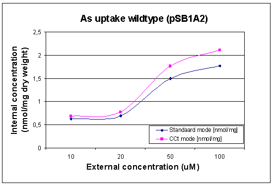
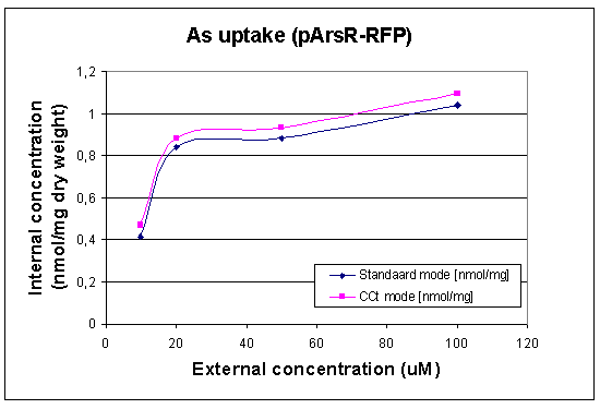
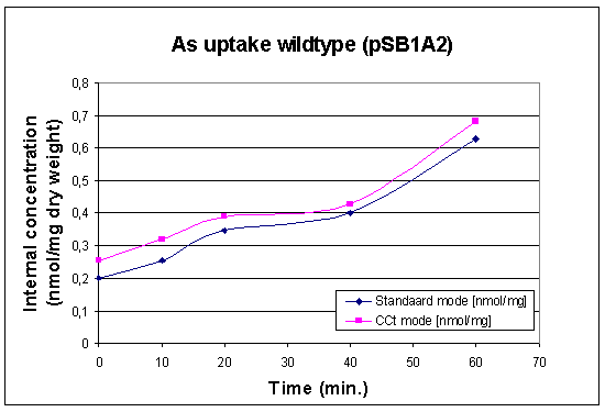
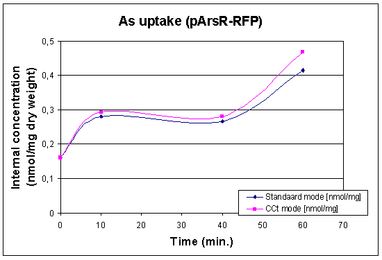
To obtain data for the optimization procedure described above we conducted ICP-MS measurements on our cells containing various devices/parts. To optimize our findings we have conducted measurements both in time and in concentration. Details on ICP-MS the experiments can be found on our Protocol Page. Measurements have been conducted at times and concentrations as indicated in the table on the right. Results can be seen below.
First Uptake Measurement
In this case we looked at the arsenic uptake of our wildtype and of our wildtype with a lot of pArs promoters with RFP. The raw data can be found at our Download Section
 | 
|
 | 
|
Getting (Vc/Vs) and other conditions
To effectively determine our constants we need to give our model some extra information. For instance what kind of constructs are inside the cel for a given experiment. Also we need to give the model the volume of cells per liter of fluid. To optain this we use the obtained dry weight and calculate how much wet weight it would have been (assuming dry weight/wet weight = 0.3) and then use the density of E. coli (1100kg/m3) to obtain the cell volume for our sample and eventually the desired volume of cells per liter.
Also we need the absolute value of Arsenic taken up by the cells in the assumption that we have one liter of sample and we know (Vc/Vs). Once we know all these parameters the optimization procedure can start.
Fluorescence Measurements
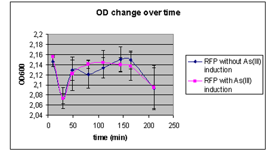
Apart from giving our model all the conditions it needs to calculate all the constants by means of the optimization procedure, we have also conducted some fluorescence measurements and made growth curves of our construct with the pArs promoter with RFP. The cells where put into a solution with either no arsenic in it or at a concentration of 100 micromolair. On the left side one can see the graph of the luminance and on right side and on the right side one can see the coresponding grow curves. The raw data of these measurements can again be found under our Downloads
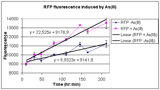 | 
|

|
Second ICPMS measurement For our second measurement I would like to refer to our Accumulation page. These measerments where higher than expected and they need further analyses before we can use them in tha characterization of our parts.
Optimization procedure
To fit our model to experimental data from different uptake experiments and/or papers we have implemented an optimization procedure that allows for experiments with different genotypes and circumstances by letting constants be overridden per experiment. It aims to optimize the sum of the RMS errors for each experiment using Simulated Annealing. By clicking the button "Fit" the optimization is started and its progress can be followed by looking at the table of constants and the graphs shown below the table (which are updated in real-time as the best solution is improved). In the optimizations procedure the ratio between v5 and K5 is kept constant. This is done because this ratio could be determined exactly using the data from the experiments done by Meng 2004 v5 itself is not fixed and may vary. (Note that in the code different experiments and graphs can be enabled/disabled, we have entered data from Kostal, Meng and our first ICP-MS measurements.)
| best | cur | gradient | solved | |
|---|---|---|---|---|
| v5/K5 | ||||
| v5 | ||||
| K5 | ||||
| k8/K7 | ||||
| k8 | ||||
| K7 | ||||
| tauBbetaB | ||||
| tauB | ||||
| betaB | ||||
| tauR | ||||
| betaRN | ||||
| tauFbetaF | ||||
| tauF | ||||
| betaF | ||||
| tauKbetaK | ||||
| tauK | ||||
| betaK | ||||
| tauGbeta5 | ||||
| tauG | ||||
| beta5 | ||||
| ars2T | ||||
| E |
|
|
|
Loading graph...
| Loading graph...
|
 "
"


