Team:EPF-Lausanne/Analysis
From 2009.igem.org
(→Maxwell-Boltzmann Energy Distribution) |
(→Maxwell-Boltzmann Energy Distribution) |
||
| Line 97: | Line 97: | ||
Fill in Start: 0, Stop at: 10, and # of bins: 100, and Apply. | Fill in Start: 0, Stop at: 10, and # of bins: 100, and Apply. | ||
| - | [[Image:Non_linear_curve_fitting.jpg|center]] | + | [[Image:Non_linear_curve_fitting.jpg|300px|center]] |
| Line 111: | Line 111: | ||
: y = (2/ sqrt(Pi * a0 ∧3 )) * sqrt(x) * exp (-x / a0) | : y = (2/ sqrt(Pi * a0 ∧3 )) * sqrt(x) * exp (-x / a0) | ||
This will fit the curve and get a fit for the parameter a0, which corresponds to kB T in units of kcal/mol. | This will fit the curve and get a fit for the parameter a0, which corresponds to kB T in units of kcal/mol. | ||
| - | [[Image: Boltzmann.png | | + | [[Image: Boltzmann.png |200px| center ]] |
'''5.''' In the Parameters drop-down menu, choose 1. You can give an initial value to A0, so that the iterations will look for a value in the vicinity of your initial guess. In the A0 window, type 0.6, which in kcal/mol corresponds to a temperature of ∼ 300K. | '''5.''' In the Parameters drop-down menu, choose 1. You can give an initial value to A0, so that the iterations will look for a value in the vicinity of your initial guess. In the A0 window, type 0.6, which in kcal/mol corresponds to a temperature of ∼ 300K. | ||
| - | [[Image:A0.jpg |center]] | + | [[Image:A0.jpg |200px|center]] |
Click on the Apply button. This will open a window with the new value for a0, as well as some statistical measures, including the Correlation Coefficient, which is a measure of the fit. | Click on the Apply button. This will open a window with the new value for a0, as well as some statistical measures, including the Correlation Coefficient, which is a measure of the fit. | ||
Revision as of 13:24, 28 July 2009
Contents |
Equilibrium
RMSD for individual residues
We aim at finding the average RMSD over time for each residue in the protein using VMD.
1. We load the .psf and .dcd files obtained after the first round of simulation.
2. In the TkCon window type:
- source residue_rmsd.tcl
- set sel_resid [[atomselect top "protein and alpha"] get resid]
This will get all the residues number of all alpha-carbons in the protein. Since there is just one and only one α-carbon per residue, it is a good option.
3. Now we will calculate the RMSD values of all atoms in the newly created selection:
- rmsd residue over time top $sel resid
At the end of the calculation, we have a list of the avergae RMSD per residue (in the file residue_rmsd.dat)
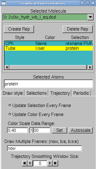
4. In VMD, in Graphics → Representations, do the following actions:
- create two replicates: protein and resname FMN in selected atoms
- for the FMN, choose CPK as a drawing method
- for the protein, choose tube as drawing method, and user as coloring method. Now click on the Trajectory tab, and in the Color Scale Data Range, type 0.40 and 1.00.
The protein is colored according to its average RMSD values. The residues displayed in blue are more mobile while the ones in red move less.
Here is a movie with the protein colored according to average RMSD values.
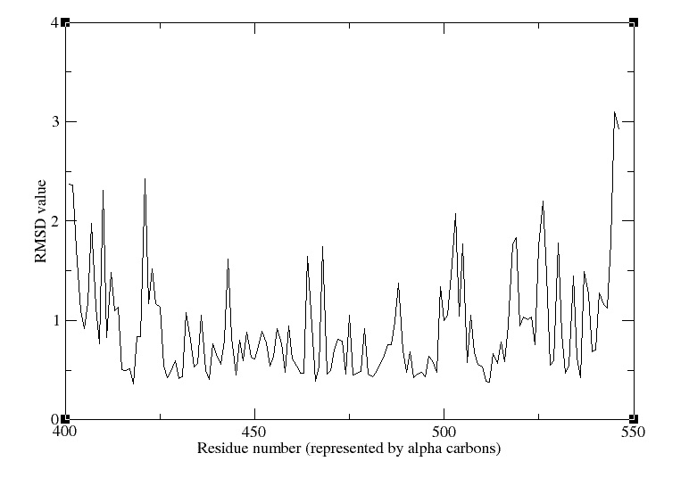
5. Now we can plot the RMSD value per residue by typing in a Terminal window :
- xmgrace residue rmsd.dat
We obtain the following picture:
Maxwell-Boltzmann Energy Distribution
Here we will confirm that the kinetic energy distribution of the atoms in a system corresponds to the Maxwell distribution for a given temperature.
1. In VMD, load the .psf file. Browse for the restart velocity file (in our case, it was 2v0w_hydr_wb_i_eq.restart.vel), the type of file need this time to be selected. In the Determine file type: pull-down menu, choose NAMD Binary Coordinates, and load again.
The molecule looks terrible! That is because VMD is reading the velocities as if they were coordinates, but how it looks doesn't matter: we just need VMD to make a file containing the masses and velocities for every atom.
2. We create a selection with all the atoms in the system, by typing in the TkCon window:
- set all [atomselect top all]
Open a file energy.dat for writing:
- set fil [open energy.dat w]
3. For each atom in the system, calculate the kinetic energy, and write it to a file
- foreach m [$all get mass] v [$all get {x y z}] {
- puts $fil [expr 0.5 * $m * [vecdot $v $v] ]
- }
Close the file:
- close $fil
All these steps can be avoided by typing in the Terminal Window:
- vmd -dispdev text -e get energy.tcl
We now have a file of raw data that can be used to fit the obtained energy distribution to the Maxwell-Boltzmann distribution. The temperature of the distribution can be obtained from that fit.
1. In a Terminal window, type xmgrace. In the xmgrace window, choose the Data → Import → ASCI I menu item. In the Files box, select the file energy.dat. Click on the OK button. You should see a black trace which correspond to the raw data.
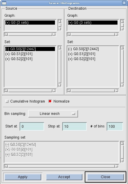
2. To look at the distribution of points, we will make a histogram of this data. Choose the Data → Transformations → Histograms menu item. In the Source → Set window, click on the first line, in order to make a histogram of the data just loaded.
Click on the Normalize option.
Fill in Start: 0, Stop at: 10, and # of bins: 100, and Apply.
3. The plot has been created, but cannot be seen yet. Use the right button of the mouse to click on the first set (in the Source → Set window).
Click on Hide. Now, go to the main Grace window and click on the button labeled AS: it will resize the plot to fit the existing values. This is the distribution of energies.
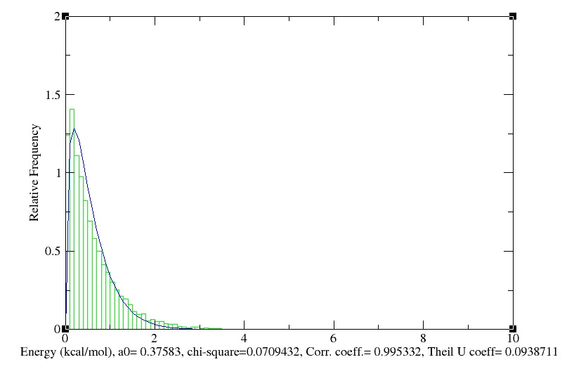
Now, we will fit a Maxwell-Boltzmann distribution to this plot and find out the temperature that the distribution corresponds to.
4. Choose the Data → Transformations → Non-linear curve fitting menu item. In the Source → Set window, click on the last line, which corresponds to the histogram you created.
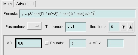
In the Main tab, type in the Formula window:
- y = (2/ sqrt(Pi * a0 ∧3 )) * sqrt(x) * exp (-x / a0)
This will fit the curve and get a fit for the parameter a0, which corresponds to kB T in units of kcal/mol.
5. In the Parameters drop-down menu, choose 1. You can give an initial value to A0, so that the iterations will look for a value in the vicinity of your initial guess. In the A0 window, type 0.6, which in kcal/mol corresponds to a temperature of ∼ 300K.
Click on the Apply button. This will open a window with the new value for a0, as well as some statistical measures, including the Correlation Coefficient, which is a measure of the fit.
The value of a0 obtained corresponds to kB T . Obtain the temperature T for this distribution with kB = 0.00198657 kcal /mol /K.
We obtwain the following histogramm!
Energies
Here we will calculate the averages of the various energies (kinetic and the different internal energies: bonded (bonds, angles and dihedrals) and non-bonded (electrostatic, van der Waals)) over the course of a simulation.
 "
"

