 "
"
Team:EPF-Lausanne/Analysis
From 2009.igem.org
(Difference between revisions)
m (→RMSD of selected atoms compared to initial position along time) |
(→Examples) |
||
| (187 intermediate revisions not shown) | |||
| Line 12: | Line 12: | ||
<br> | <br> | ||
| - | |||
| - | |||
| - | |||
| + | =Scripts= | ||
| + | As this page is getting crowded, we created another page to explain all the scripts we wrote. The current page has some kind of step by step tutorials, but if you want fast informations, you better go to the [[Team:EPF-Lausanne/Scripts|script page]]. | ||
| - | |||
| - | |||
| - | |||
| - | |||
| + | =Tutorials= | ||
| + | <br> | ||
| + | == Maxwell-Boltzmann Energy Distribution == | ||
| - | + | <html> | |
| - | + | <script type="text/javascript" language="JavaScript"><!-- | |
| - | + | function HideContent(d) { | |
| + | document.getElementById(d).style.display = "none"; | ||
| + | } | ||
| + | function ShowContent(d) { | ||
| + | document.getElementById(d).style.display = "block"; | ||
| + | } | ||
| + | function ReverseDisplay(d) { | ||
| + | if(document.getElementById(d).style.display == "none") { document.getElementById(d).style.display = "block"; } | ||
| + | else { document.getElementById(d).style.display = "none"; } | ||
| + | } | ||
| + | //--></script> | ||
| + | <p> | ||
| + | <a href="javascript:ReverseDisplay('hs1')"> Click here to show/hide</a> | ||
| + | </p> | ||
| - | + | <div id="hs1" style="display:none;"> | |
| - | + | <p> | |
| - | + | Here we will confirm that the kinetic energy distribution of the atoms in a system corresponds to the Maxwell distribution for a given temperature. | |
| - | * | + | <br><br> |
| + | <b>1.</b> In VMD, load the <i>.psf file</i>. Browse for the restart velocity file (in our case, it was <i>2v0w_hydr_wb_i_eq.restart.vel</i>), the type of file need this time to be selected. In the Determine file type: pull-down menu, choose NAMD Binary Coordinates, and load again. | ||
| + | <br> | ||
| + | The molecule looks terrible! That is because VMD is reading the velocities as if they were coordinates, but how it looks doesn't matter: we just need VMD to make a file containing the masses and velocities for every atom. | ||
| + | <br><br> | ||
| + | <b>2.</b> We create a selection with all the atoms in the system, by typing in the TkCon window: | ||
| + | <br><span style="font-family: Courier;"> set all [atomselect top all] </span> | ||
| + | <br> Open a file energy.dat for writing: | ||
| + | <br><span style="font-family: Courier;"> set fil [open energy.dat w] </span> | ||
| + | <br><br> | ||
| + | <b>3.</b> For each atom in the system, calculate the kinetic energy, and write it to a file : | ||
| + | <br><span style="font-family: Courier;"> foreach m [$all get mass] v [$all get {x y z}] { | ||
| + | <br> puts $fil [expr 0.5 * $m * [vecdot $v $v] ] | ||
| + | <br> } </span> | ||
| + | <br>Close the file: | ||
| + | <br><span style="font-family: Courier;"> close $fil </span> | ||
| + | <br> | ||
| + | <br>All these steps can be avoided by typing in the Terminal Window: | ||
| + | <br><span style="font-family: Courier;"> vmd -dispdev text -e get energy.tcl </span> | ||
| + | <br> | ||
| + | <br>We now have a file of raw data that can be used to fit the obtained energy distribution to the Maxwell-Boltzmann distribution. The temperature of the distribution can be obtained from that fit. | ||
| + | <br><br> | ||
| + | <b>1.</b> In a Terminal window, type xmgrace. In the xmgrace window, choose the Data → Import → ASCI I menu item. In the Files box, select the file <i>energy.dat</i>. Click on the OK button. You should see a black trace which correspond to the raw data. | ||
| + | <br><br> | ||
| + | <b>2.</b> To look at the distribution of points, we will make a histogram of this data. Choose the Data → Transformations → Histograms menu item. In the Source → Set window, click on the first line, in order to make a histogram of the data just loaded. | ||
| + | <br> | ||
| + | Click on the Normalize option. | ||
| + | <br> | ||
| + | Fill in Start: 0, Stop at: 10, and # of bins: 100, and Apply. | ||
| + | <br> | ||
| + | <center> | ||
| + | <img src="https://static.igem.org/mediawiki/2009/thumb/8/8c/Non_linear_curve_fitting.jpg/300px-Non_linear_curve_fitting.jpg"> | ||
| + | </center><br> | ||
| + | <b>3.</b> The plot has been created, but cannot be seen yet. Use the right button of the mouse to click on the first set (in the Source → Set window). | ||
| + | <br>Click on Hide. Now, go to the main Grace window and click on the button labeled AS: it will resize the plot to fit the existing values. This is the distribution of energies. | ||
| + | <br> | ||
| + | Now, we will fit a Maxwell-Boltzmann distribution to this plot and find out the temperature that the distribution corresponds to. | ||
| + | <br><br> | ||
| + | <b>4.</b> Choose the Data → Transformations → Non-linear curve fitting menu item. In the Source → Set window, click on the last line, which corresponds to the histogram you created. | ||
| + | <br> | ||
| + | <br>In the Main tab, type in the Formula window: | ||
| + | <br><span style="font-family: Courier;"> y = (2/ sqrt(Pi * a0 ∧3 )) * sqrt(x) * exp (-x / a0) </span> | ||
| + | <br>This will fit the curve and get a fit for the parameter a0, which corresponds to kB T in units of kcal/mol. | ||
| + | <br><center><img src="https://static.igem.org/mediawiki/2009/thumb/a/a1/Boltzmann.png/300px-Boltzmann.png"></center> | ||
| + | <br> | ||
| + | <b>5.</b> In the Parameters drop-down menu, choose 1. You can give an initial value to A0, so that the iterations will look for a value in the vicinity of your initial guess. In the A0 window, type 0.6, which in kcal/mol corresponds to a temperature of ∼ 300K. | ||
| + | <br><center><img src="https://static.igem.org/mediawiki/2009/thumb/0/04/A0.jpg/350px-A0.jpg"></center> | ||
| + | <br>Click on the Apply button. This will open a window with the new value for a0, as well as some statistical measures, including the Correlation Coefficient, which is a measure of the fit. | ||
| + | <br><center><img src="https://static.igem.org/mediawiki/2009/thumb/9/92/Correlation_coefficient.jpg/350px-Correlation_coefficient.jpg"></center> | ||
| + | <br>The value of a0 obtained corresponds to kB T . Obtain the temperature T for this distribution with kB = 0.00198657 kcal | ||
| + | /mol /K. | ||
| + | <br> | ||
| + | We obtain the following histogramm! | ||
| + | <br><center><img src="https://static.igem.org/mediawiki/2009/a/aa/Maxwell-Boltzmann_Energy_Distribution.jpg"></center> | ||
| + | <br> | ||
| - | |||
| - | + | <html> | |
| + | <p align="center" class="style1"><a href="#top"><img src="https://static.igem.org/mediawiki/2009/thumb/0/06/Up_arrow.png/50px-Up_arrow.png" alt="Back to top" border="0"></a><br></p> | ||
| + | </html> | ||
| + | <br> | ||
| + | <html><center> | ||
| + | <style type="text/css"> | ||
| + | <!-- | ||
| + | .combobox { | ||
| + | background-color: #FFFFFF; | ||
| + | color: #808080; | ||
| + | font-size: 10pt; | ||
| + | font-family: verdana; | ||
| + | font-weight: bold; | ||
| + | } | ||
| + | --> | ||
| + | </style> | ||
| + | <form> | ||
| + | <table border="0" width="80" cellspacing="0"> | ||
| + | <tr><td width="100%" bgcolor="#000000"> | ||
| + | <table border="0" width="100%" cellspacing="0" cellpadding="0"> | ||
| + | <tr><td width="100%" background="https://static.igem.org/mediawiki/2009/b/b3/BoxtopA.png"><img border="0" src="11dot.gif" width="19" height="19"></td></tr> | ||
| + | </table> | ||
| + | <table border="0" width="100%" cellspacing="0" cellpadding="3"> | ||
| + | <tr><td width="2%" background="https://static.igem.org/mediawiki/2009/b/bd/BoxbackA.png"> | ||
| + | <img border="0" src="11dot.gif" width="18" height="18"> | ||
| + | </td><td width="98%" background="https://static.igem.org/mediawiki/2009/6/6e/BoxbackB.png"> | ||
| + | <select class="combobox" name="SiteMap" onchange="if(options[selectedIndex].value){location = options[selectedIndex].value}" size="1"> | ||
| + | <option selected>Go to: </option> | ||
| + | <option value="https://2009.igem.org/Team:EPF-Lausanne/Analysis#Maxwell-Boltzmann_Energy_Distribution">Maxwell-Boltzmann Energy Distribution </option><option value="https://2009.igem.org/Team:EPF-Lausanne/Analysis#Energies">Energies</option><option value="https://2009.igem.org/Team:EPF-Lausanne/Analysis#Temperature_distribution">Temperature distribution</option><option value="https://2009.igem.org/Team:EPF-Lausanne/Analysis#Density">Density </option><option value="https://2009.igem.org/Team:EPF-Lausanne/Analysis#Pressure_as_a_function_of_simulation_time">Pressure</option><option value="https://2009.igem.org/Team:EPF-Lausanne/Analysis#RMSD_for_individual_residues">RMSD for individual residues</option><option value="https://2009.igem.org/Team:EPF-Lausanne/Analysis#RMSD_of_selected_atoms_compared_to_initial_position_along_time">RMSD of selected atoms</option><option value="https://2009.igem.org/Team:EPF-Lausanne/Analysis#Salt_bridges">Salt bridges</option><option value="https://2009.igem.org/Team:EPF-Lausanne/Analysis#RMSF">RMSF</option> | ||
| + | </select> | ||
| + | </td></tr> | ||
| + | </table> | ||
| + | </td></tr> | ||
| + | </table> | ||
| + | </form></center> | ||
| - | + | </p> | |
| + | </div> | ||
| + | </html> | ||
| + | <br> | ||
| - | + | == Energies == | |
| + | <html> | ||
| + | <script type="text/javascript" language="JavaScript"><!-- | ||
| + | function HideContent(d) { | ||
| + | document.getElementById(d).style.display = "none"; | ||
| + | } | ||
| + | function ShowContent(d) { | ||
| + | document.getElementById(d).style.display = "block"; | ||
| + | } | ||
| + | function ReverseDisplay(d) { | ||
| + | if(document.getElementById(d).style.display == "none") { document.getElementById(d).style.display = "block"; } | ||
| + | else { document.getElementById(d).style.display = "none"; } | ||
| + | } | ||
| + | //--></script> | ||
| - | '' | + | <p> |
| - | + | <a href="javascript:ReverseDisplay('hs2')"> Click here to show/hide</a> | |
| - | + | </p> | |
| - | + | <div id="hs2" style="display:none;"> | |
| - | + | <p> | |
| - | + | Here we will calculate the averages of the various energies (kinetic and the different internal energies: bonded (bonds, | |
| - | + | angles and dihedrals) and non-bonded (electrostatic, van der Waals)) over the course of a simulation. | |
| - | </html> | + | <br><br> |
| + | <b>1.</b> We start with a file obtained from NAMD: <br>http://www.ks.uiuc.edu/Research/namd/utilities/ and download <i>namdstat.tcl</i> | ||
| + | <br><br> | ||
| + | <b>2.</b> In the VMD TkCon window, type : | ||
| + | <br><span style="font-family: Courier;"> source namdstats.tcl | ||
| + | <br> data avg ../namd_log 101 last </span> | ||
| + | <br>The second line will call a procedure which will calculate the average for all output variables in the log file from the first logged timestep after 101 to the end of the simulation. | ||
| + | </p> | ||
| + | </div> | ||
| + | </html> | ||
<br> | <br> | ||
| + | == Temperature distribution == | ||
| + | <html> | ||
| + | <script type="text/javascript" language="JavaScript"><!-- | ||
| + | function HideContent(d) { | ||
| + | document.getElementById(d).style.display = "none"; | ||
| + | } | ||
| + | function ShowContent(d) { | ||
| + | document.getElementById(d).style.display = "block"; | ||
| + | } | ||
| + | function ReverseDisplay(d) { | ||
| + | if(document.getElementById(d).style.display == "none") { document.getElementById(d).style.display = "block"; } | ||
| + | else { document.getElementById(d).style.display = "none"; } | ||
| + | } | ||
| + | //--></script> | ||
| - | + | <p> | |
| - | + | <a href="javascript:ReverseDisplay('hs3')"> Click here to show/hide</a> | |
| + | </p> | ||
| - | + | <div id="hs3" style="display:none;"> | |
| + | <p> | ||
| - | + | <b>Objective:</b> Simulate our protein in an NVE ensemble, and analyze the temperature distribution. | |
| + | <br> | ||
| + | <br>In order to obtain the data for the temperature from the log file we will again use the script <i>namdstats.tcl</i>, which was already sourced. Type in a terminal window: | ||
| + | <br><span style="font-family: Courier;"> data_time TEMP namd_log </span> | ||
| + | <br>It will store each timestep and its corresponding temperature in the file TEMP.dat. | ||
| + | <br><br> | ||
| + | Using EXCEL, we obtain the following graph, which represents the evolution of the temperature in function of time: | ||
| + | <br><br><img src="https://static.igem.org/mediawiki/2009/c/cf/Temp%28t%29.png"> | ||
| + | <br>The first part corresponds the the heating, then we let the system reach an equilibrium (NPT state), a NVT portion, and finally a NPT portion again. | ||
| - | + | <html><center> | |
| - | : | + | <style type="text/css"> |
| - | + | <!-- | |
| - | : | + | .combobox { |
| + | background-color: #FFFFFF; | ||
| + | color: #808080; | ||
| + | font-size: 10pt; | ||
| + | font-family: verdana; | ||
| + | font-weight: bold; | ||
| + | } | ||
| + | --> | ||
| + | </style> | ||
| + | <form> | ||
| + | <table border="0" width="80" cellspacing="0"> | ||
| + | <tr><td width="100%" bgcolor="#000000"> | ||
| + | <table border="0" width="100%" cellspacing="0" cellpadding="0"> | ||
| + | <tr><td width="100%" background="https://static.igem.org/mediawiki/2009/b/b3/BoxtopA.png"><img border="0" src="11dot.gif" width="19" height="19"></td></tr> | ||
| + | </table> | ||
| + | <table border="0" width="100%" cellspacing="0" cellpadding="3"> | ||
| + | <tr><td width="2%" background="https://static.igem.org/mediawiki/2009/b/bd/BoxbackA.png"> | ||
| + | <img border="0" src="11dot.gif" width="18" height="18"> | ||
| + | </td><td width="98%" background="https://static.igem.org/mediawiki/2009/6/6e/BoxbackB.png"> | ||
| + | <select class="combobox" name="SiteMap" onchange="if(options[selectedIndex].value){location = options[selectedIndex].value}" size="1"> | ||
| + | <option selected>Go to: </option> | ||
| + | <option value="https://2009.igem.org/Team:EPF-Lausanne/Analysis#Maxwell-Boltzmann_Energy_Distribution">Maxwell-Boltzmann Energy Distribution </option><option value="https://2009.igem.org/Team:EPF-Lausanne/Analysis#Energies">Energies</option><option value="https://2009.igem.org/Team:EPF-Lausanne/Analysis#Temperature_distribution">Temperature distribution</option><option value="https://2009.igem.org/Team:EPF-Lausanne/Analysis#Density">Density </option><option value="https://2009.igem.org/Team:EPF-Lausanne/Analysis#Pressure_as_a_function_of_simulation_time">Pressure</option><option value="https://2009.igem.org/Team:EPF-Lausanne/Analysis#RMSD_for_individual_residues">RMSD for individual residues</option><option value="https://2009.igem.org/Team:EPF-Lausanne/Analysis#RMSD_of_selected_atoms_compared_to_initial_position_along_time">RMSD of selected atoms</option><option value="https://2009.igem.org/Team:EPF-Lausanne/Analysis#Salt_bridges">Salt bridges</option><option value="https://2009.igem.org/Team:EPF-Lausanne/Analysis#RMSF">RMSF</option> | ||
| + | </select> | ||
| + | </td></tr> | ||
| + | </table> | ||
| + | </td></tr> | ||
| + | </table> | ||
| + | </form></center> | ||
| + | </p> | ||
| + | </div> | ||
| + | </html> | ||
| + | <br> | ||
| - | + | == Density == | |
| - | + | ||
| - | + | ||
| - | + | ||
| - | + | ||
| - | + | ||
| + | <html> | ||
| + | <script type="text/javascript" language="JavaScript"><!-- | ||
| + | function HideContent(d) { | ||
| + | document.getElementById(d).style.display = "none"; | ||
| + | } | ||
| + | function ShowContent(d) { | ||
| + | document.getElementById(d).style.display = "block"; | ||
| + | } | ||
| + | function ReverseDisplay(d) { | ||
| + | if(document.getElementById(d).style.display == "none") { document.getElementById(d).style.display = "block"; } | ||
| + | else { document.getElementById(d).style.display = "none"; } | ||
| + | } | ||
| + | //--></script> | ||
| - | + | <p> | |
| - | : | + | <a href="javascript:ReverseDisplay('hs4')"> Click here to show/hide</a> |
| + | </p> | ||
| + | <div id="hs4" style="display:none;"> | ||
| + | <p> | ||
| - | + | In order to obtain the data for the volume from the log file we will again use the script ''namdstats.tcl'', which was already sourced. Type in a terminal window: | |
| + | <br><span style="font-family: Courier;"> data_time VOLUME namd_log </span> | ||
| + | <br>It will store each timestep and its corresponding temperature in the file TEMP.dat. | ||
| + | <br><br> | ||
| + | Using EXCEL, we obtain the following graph, which represents the evolution of the density in function of time: | ||
| + | <br><center><img src="https://static.igem.org/mediawiki/2009/e/e7/Density.jpg"></center> | ||
| + | <br>The first part corresponds the the heating, then we let the system reach an equilibrium (NPT state), a NVT portion, and finally a NPT portion again. | ||
| + | <html><center> | ||
| + | <style type="text/css"> | ||
| + | <!-- | ||
| + | .combobox { | ||
| + | background-color: #FFFFFF; | ||
| + | color: #808080; | ||
| + | font-size: 10pt; | ||
| + | font-family: verdana; | ||
| + | font-weight: bold; | ||
| + | } | ||
| + | --> | ||
| + | </style> | ||
| + | <form> | ||
| + | <table border="0" width="80" cellspacing="0"> | ||
| + | <tr><td width="100%" bgcolor="#000000"> | ||
| + | <table border="0" width="100%" cellspacing="0" cellpadding="0"> | ||
| + | <tr><td width="100%" background="https://static.igem.org/mediawiki/2009/b/b3/BoxtopA.png"><img border="0" src="11dot.gif" width="19" height="19"></td></tr> | ||
| + | </table> | ||
| + | <table border="0" width="100%" cellspacing="0" cellpadding="3"> | ||
| + | <tr><td width="2%" background="https://static.igem.org/mediawiki/2009/b/bd/BoxbackA.png"> | ||
| + | <img border="0" src="11dot.gif" width="18" height="18"> | ||
| + | </td><td width="98%" background="https://static.igem.org/mediawiki/2009/6/6e/BoxbackB.png"> | ||
| + | <select class="combobox" name="SiteMap" onchange="if(options[selectedIndex].value){location = options[selectedIndex].value}" size="1"> | ||
| + | <option selected>Go to: </option> | ||
| + | <option value="https://2009.igem.org/Team:EPF-Lausanne/Analysis#Maxwell-Boltzmann_Energy_Distribution">Maxwell-Boltzmann Energy Distribution </option><option value="https://2009.igem.org/Team:EPF-Lausanne/Analysis#Energies">Energies</option><option value="https://2009.igem.org/Team:EPF-Lausanne/Analysis#Temperature_distribution">Temperature distribution</option><option value="https://2009.igem.org/Team:EPF-Lausanne/Analysis#Density">Density </option><option value="https://2009.igem.org/Team:EPF-Lausanne/Analysis#Pressure_as_a_function_of_simulation_time">Pressure</option><option value="https://2009.igem.org/Team:EPF-Lausanne/Analysis#RMSD_for_individual_residues">RMSD for individual residues</option><option value="https://2009.igem.org/Team:EPF-Lausanne/Analysis#RMSD_of_selected_atoms_compared_to_initial_position_along_time">RMSD of selected atoms</option><option value="https://2009.igem.org/Team:EPF-Lausanne/Analysis#Salt_bridges">Salt bridges</option><option value="https://2009.igem.org/Team:EPF-Lausanne/Analysis#RMSF">RMSF</option> | ||
| + | </select> | ||
| + | </td></tr> | ||
| + | </table> | ||
| + | </td></tr> | ||
| + | </table> | ||
| + | </form></center> | ||
| - | + | </p> | |
| + | </div> | ||
| + | </html> | ||
| + | <br> | ||
| + | == Pressure as a function of simulation time == | ||
| - | + | <html> | |
| + | <script type="text/javascript" language="JavaScript"><!-- | ||
| + | function HideContent(d) { | ||
| + | document.getElementById(d).style.display = "none"; | ||
| + | } | ||
| + | function ShowContent(d) { | ||
| + | document.getElementById(d).style.display = "block"; | ||
| + | } | ||
| + | function ReverseDisplay(d) { | ||
| + | if(document.getElementById(d).style.display == "none") { document.getElementById(d).style.display = "block"; } | ||
| + | else { document.getElementById(d).style.display = "none"; } | ||
| + | } | ||
| + | //--></script> | ||
| - | Click | + | <p> |
| + | <a href="javascript:ReverseDisplay('hs5')"> Click here to show/hide</a> | ||
| + | </p> | ||
| - | + | <div id="hs5" style="display:none;"> | |
| + | <p> | ||
| - | + | In order to obtain the data for the pressure from the log file we will again use the script <i>namdstats.tcl</i>, which has been updated for the occasion. | |
| + | <br>The file can be found <a href="https://static.igem.org/mediawiki/2009/6/67/Namdstats_igem09.txt"> here </a>. Please rename to namdstats<b>.tcl</b> after download. | ||
| + | <br><br> | ||
| + | Here are the steps to use this script: | ||
| + | <br><span style="font-family: Courier;"> source namdstats.tcl | ||
| + | <br> data_time DATA_NAME LOG_FILE </span> | ||
| + | <br>It will extract data from LOG_FILE, creating a DATA_NAME.dat containing values and time informations. | ||
| + | <br><br> | ||
| + | Available DATA_NAME can be: BOND, ANGLE, DIHED, IMPRP, ELECT, VDW, BOUNDARY, MISC, KINETIC, TOTAL, TEMP, TOTAL2, TOTAL3, TEMPAVG, PRESSURE, GPRESSURE, VOLUME, PRESSAVG, GPRESSAVG. | ||
| + | <br><br> | ||
| + | So, to extract pressure from our first simulation, the command is: data_time PRESSURE namd_log | ||
| + | <br><br> | ||
| + | Here is a small plot of pressure and temperature in function of time | ||
| + | <img src="https://static.igem.org/mediawiki/2009/f/f9/1st_run.jpg"> | ||
| + | <html><center> | ||
| + | <style type="text/css"> | ||
| + | <!-- | ||
| + | .combobox { | ||
| + | background-color: #FFFFFF; | ||
| + | color: #808080; | ||
| + | font-size: 10pt; | ||
| + | font-family: verdana; | ||
| + | font-weight: bold; | ||
| + | } | ||
| + | --> | ||
| + | </style> | ||
| + | <form> | ||
| + | <table border="0" width="80" cellspacing="0"> | ||
| + | <tr><td width="100%" bgcolor="#000000"> | ||
| + | <table border="0" width="100%" cellspacing="0" cellpadding="0"> | ||
| + | <tr><td width="100%" background="https://static.igem.org/mediawiki/2009/b/b3/BoxtopA.png"><img border="0" src="11dot.gif" width="19" height="19"></td></tr> | ||
| + | </table> | ||
| + | <table border="0" width="100%" cellspacing="0" cellpadding="3"> | ||
| + | <tr><td width="2%" background="https://static.igem.org/mediawiki/2009/b/bd/BoxbackA.png"> | ||
| + | <img border="0" src="11dot.gif" width="18" height="18"> | ||
| + | </td><td width="98%" background="https://static.igem.org/mediawiki/2009/6/6e/BoxbackB.png"> | ||
| + | <select class="combobox" name="SiteMap" onchange="if(options[selectedIndex].value){location = options[selectedIndex].value}" size="1"> | ||
| + | <option selected>Go to: </option> | ||
| + | <option value="https://2009.igem.org/Team:EPF-Lausanne/Analysis#Maxwell-Boltzmann_Energy_Distribution">Maxwell-Boltzmann Energy Distribution </option><option value="https://2009.igem.org/Team:EPF-Lausanne/Analysis#Energies">Energies</option><option value="https://2009.igem.org/Team:EPF-Lausanne/Analysis#Temperature_distribution">Temperature distribution</option><option value="https://2009.igem.org/Team:EPF-Lausanne/Analysis#Density">Density </option><option value="https://2009.igem.org/Team:EPF-Lausanne/Analysis#Pressure_as_a_function_of_simulation_time">Pressure</option><option value="https://2009.igem.org/Team:EPF-Lausanne/Analysis#RMSD_for_individual_residues">RMSD for individual residues</option><option value="https://2009.igem.org/Team:EPF-Lausanne/Analysis#RMSD_of_selected_atoms_compared_to_initial_position_along_time">RMSD of selected atoms</option><option value="https://2009.igem.org/Team:EPF-Lausanne/Analysis#Salt_bridges">Salt bridges</option><option value="https://2009.igem.org/Team:EPF-Lausanne/Analysis#RMSF">RMSF</option> | ||
| + | </select> | ||
| + | </td></tr> | ||
| + | </table> | ||
| + | </td></tr> | ||
| + | </table> | ||
| + | </form></center> | ||
| - | + | </p> | |
| - | + | </div> | |
| + | </html> | ||
| + | <br> | ||
| - | + | ==RMSD for individual residues== | |
| + | <html> | ||
| + | <script type="text/javascript" language="JavaScript"><!-- | ||
| + | function HideContent(d) { | ||
| + | document.getElementById(d).style.display = "none"; | ||
| + | } | ||
| + | function ShowContent(d) { | ||
| + | document.getElementById(d).style.display = "block"; | ||
| + | } | ||
| + | function ReverseDisplay(d) { | ||
| + | if(document.getElementById(d).style.display == "none") { document.getElementById(d).style.display = "block"; } | ||
| + | else { document.getElementById(d).style.display = "none"; } | ||
| + | } | ||
| + | //--></script> | ||
| - | '' | + | <p> |
| + | <a href="javascript:ReverseDisplay('hs6')"> Click here to show/hide</a> | ||
| + | </p> | ||
| - | + | <div id="hs6" style="display:none;"> | |
| - | + | <p> | |
| - | + | ||
| - | + | ||
| + | We aim at finding the average RMSD over time for each residue in the protein using VMD. | ||
| + | <br> | ||
| + | <b>1.</b> We load the <i>.psf</i> and <i>.dcd</i> files obtained after the first round of simulation. | ||
| + | <br><br> | ||
| + | <b>2.</b> In the TkCon window type: | ||
| + | <br><span style="font-family: Courier;"> source residue_rmsd.tcl | ||
| + | <br> set sel_resid [[atomselect top "protein and alpha"] get resid] </span> | ||
| + | <br> | ||
| + | <br>This will get all the residues number of all alpha-carbons in the protein. Since there is just one and only one α-carbon per residue, it is a good option. | ||
| + | <br><br> | ||
| + | <b>3.</b> Now we will calculate the RMSD values of all atoms in the newly created selection: | ||
| + | <br><span style="font-family: Courier;"> rmsd_residue_over_time top $sel resid </span> | ||
| + | <br>At the end of the calculation, we have a list of the avergae RMSD per residue (in the file residue_rmsd.dat) | ||
| + | <br> | ||
| + | <br><b>Remark</b>: we updated <a href="https://static.igem.org/mediawiki/2009/1/1f/Residue_rmsd_v2.txt"> the script residue_rmsd.tcl</a> to be able to specify on which frames the rsmd has to be computed. Please have a look on this wiki for a more up-to-date version of the file... Command is: | ||
| + | <br><span style="font-family: Courier;"> rmsd_residue_over_time top $sel resid FIRST_FRAME LAST_FRAME </span> | ||
| + | <br><br> | ||
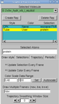
| + | <b>4.</b> In VMD, in Graphics → Representations, do the following actions: | ||
| + | <ul> | ||
| + | <li> create two replicates: protein and resname FMN in selected atoms | ||
| + | <li> for the FMN, choose CPK as a drawing method | ||
| + | <li> for the protein, choose tube as drawing method, and <i>user</i> as coloring method. Now click on the Trajectory tab, and in the Color Scale Data Range, type 0.40 and 1.00. | ||
| + | </ul><br><center> | ||
| + | <img src="https://static.igem.org/mediawiki/2009/thumb/d/dd/Vmd_color.png/200px-Vmd_color.png"></center> | ||
| + | <br><br> | ||
| + | The protein is colored according to its average RMSD values. The residues displayed in blue are more mobile while the ones in red move less. | ||
| + | <br><br> | ||
| + | Here is a movie with the protein colored according to average RMSD values: <a href="https://static.igem.org/mediawiki/2009/4/4d/Moving_residue.mov"> video </a> | ||
| + | <br> | ||
| - | + | <br><br> | |
| + | <b>5.</b> Now we can plot the RMSD value per residue by typing in a Terminal window : | ||
| + | <br><span style="font-family: Courier;"> xmgrace residue rmsd.dat </span> | ||
| + | <br>We obtain the following picture: | ||
| + | <br> | ||
| + | <img src="https://static.igem.org/mediawiki/2009/thumb/c/cc/RMSD_CA_per_res.jpg/700px-RMSD_CA_per_res.jpg"> | ||
| + | <br> | ||
| - | + | <hr/> | |
| + | <p align="center"><big> <b>RMSD of residue within 3 angström of the FMN</b> </big></p> | ||
| - | + | <img src="https://static.igem.org/mediawiki/2009/6/6c/Resid_3A.jpg"> | |
| + | <br><br> | ||
| + | We can see that the residues that move the most are the residue number: 425, 451, 453 | ||
| - | + | <br><br> | |
| - | + | <hr/> | |
| - | / | + | <p align="center"><big> <b>RMSD of residue within 6 angström of the FMN</b> </big></p> |
| + | <img src="https://static.igem.org/mediawiki/2009/3/3e/Resid_6A.jpg"> | ||
| + | <br> | ||
| + | We can see that the residues that move the most are the residue number: 424, 425, 464, 468 | ||
| + | <br> | ||
| - | |||
| - | |||
| - | |||
| - | |||
<p align="center" class="style1"><a href="#top"><img src="https://static.igem.org/mediawiki/2009/thumb/0/06/Up_arrow.png/50px-Up_arrow.png" alt="Back to top" border="0"></a><br></p> | <p align="center" class="style1"><a href="#top"><img src="https://static.igem.org/mediawiki/2009/thumb/0/06/Up_arrow.png/50px-Up_arrow.png" alt="Back to top" border="0"></a><br></p> | ||
| - | |||
<br> | <br> | ||
| - | == | + | <html><center> |
| - | + | <style type="text/css"> | |
| - | + | <!-- | |
| + | .combobox { | ||
| + | background-color: #FFFFFF; | ||
| + | color: #808080; | ||
| + | font-size: 10pt; | ||
| + | font-family: verdana; | ||
| + | font-weight: bold; | ||
| + | } | ||
| + | --> | ||
| + | </style> | ||
| + | <form> | ||
| + | <table border="0" width="80" cellspacing="0"> | ||
| + | <tr><td width="100%" bgcolor="#000000"> | ||
| + | <table border="0" width="100%" cellspacing="0" cellpadding="0"> | ||
| + | <tr><td width="100%" background="https://static.igem.org/mediawiki/2009/b/b3/BoxtopA.png"><img border="0" src="11dot.gif" width="19" height="19"></td></tr> | ||
| + | </table> | ||
| + | <table border="0" width="100%" cellspacing="0" cellpadding="3"> | ||
| + | <tr><td width="2%" background="https://static.igem.org/mediawiki/2009/b/bd/BoxbackA.png"> | ||
| + | <img border="0" src="11dot.gif" width="18" height="18"> | ||
| + | </td><td width="98%" background="https://static.igem.org/mediawiki/2009/6/6e/BoxbackB.png"> | ||
| + | <select class="combobox" name="SiteMap" onchange="if(options[selectedIndex].value){location = options[selectedIndex].value}" size="1"> | ||
| + | <option selected>Go to: </option> | ||
| + | <option value="https://2009.igem.org/Team:EPF-Lausanne/Analysis#Maxwell-Boltzmann_Energy_Distribution">Maxwell-Boltzmann Energy Distribution </option><option value="https://2009.igem.org/Team:EPF-Lausanne/Analysis#Energies">Energies</option><option value="https://2009.igem.org/Team:EPF-Lausanne/Analysis#Temperature_distribution">Temperature distribution</option><option value="https://2009.igem.org/Team:EPF-Lausanne/Analysis#Density">Density </option><option value="https://2009.igem.org/Team:EPF-Lausanne/Analysis#Pressure_as_a_function_of_simulation_time">Pressure</option><option value="https://2009.igem.org/Team:EPF-Lausanne/Analysis#RMSD_for_individual_residues">RMSD for individual residues</option><option value="https://2009.igem.org/Team:EPF-Lausanne/Analysis#RMSD_of_selected_atoms_compared_to_initial_position_along_time">RMSD of selected atoms</option><option value="https://2009.igem.org/Team:EPF-Lausanne/Analysis#Salt_bridges">Salt bridges</option><option value="https://2009.igem.org/Team:EPF-Lausanne/Analysis#RMSF">RMSF</option> | ||
| + | </select> | ||
| + | </td></tr> | ||
| + | </table> | ||
| + | </td></tr> | ||
| + | </table> | ||
| + | </form></center> | ||
| + | </p> | ||
| + | </div> | ||
| + | </html> | ||
| + | <br> | ||
| - | + | == RMSD of selected atoms compared to initial position along time == | |
| + | <html> | ||
| + | <script type="text/javascript" language="JavaScript"><!-- | ||
| + | function HideContent(d) { | ||
| + | document.getElementById(d).style.display = "none"; | ||
| + | } | ||
| + | function ShowContent(d) { | ||
| + | document.getElementById(d).style.display = "block"; | ||
| + | } | ||
| + | function ReverseDisplay(d) { | ||
| + | if(document.getElementById(d).style.display == "none") { document.getElementById(d).style.display = "block"; } | ||
| + | else { document.getElementById(d).style.display = "none"; } | ||
| + | } | ||
| + | //--></script> | ||
| - | '' | + | <p> |
| - | + | <a href="javascript:ReverseDisplay('hs7')"> Click here to show/hide</a> | |
| - | + | </p> | |
| - | + | ||
| + | <div id="hs7" style="display:none;"> | ||
| + | <p> | ||
| - | = | + | <b>This script was highly updated, please go to the <a href="https://2009.igem.org/Team:EPF-Lausanne/Scripts">script page</a> if you encounter a problem!!! |
| - | + | ||
| - | + | <br>Selections are not precise here!</b> | |
| - | + | <br><br> | |
| - | + | ||
| + | We made a small TCL script to calculate RMSD from selected atoms compared to their initial position along timestep. | ||
| + | The file can be found <a href="https://static.igem.org/mediawiki/2009/a/ad/Residue_rmsd_igem09.txt">here</a>. Please rename to Residue_rmsd_igem09<b>.tcl</b> after download. | ||
| + | <br><br> | ||
| + | Example to run the script: | ||
| + | <br><span style="font-family: Courier;"> load ''.dcd'' + ''.psf'' on VMD | ||
| + | <br> source residue_rmsd_igem09.tcl | ||
| + | <br> set sel_resid [[atomselect top "protein and alpha"] get resid] | ||
| + | <br> rmsd_residue_over_time top $sel_resid 0 0 </span> | ||
| + | <br><br> | ||
| + | We tried to select only backbone from protein + FMN → change | ||
| + | <br><span style="font-family: Courier;"> <i>set sel_resid [[atomselect top "backbone"] get resid] </i></span> | ||
| + | <br><br> | ||
| + | <b>The script was updated to be able to define reference frame and first frame were RMSD will be calculated.</b> We usually don't need to compute RMSD during heating, for instance. RMSD takes a lot of time. In our first run 1 frame = 100 timesteps * 2 fs*timesteps^-1 = 200 fs | ||
| + | <br><br> | ||
| + | complete form for run is: | ||
| + | <br><span style="font-family: Courier;"> <i>rmsd_residue_over_time top $sel_resid FIRST_FRAME REFERENCE_FRAME</i></span> | ||
| + | <br><br> | ||
| + | For our first run, if we want to select only the 295°K NPT plateau, and set its first frame as reference, we have to launch: | ||
| + | <br><span style="font-family: Courier;"> <i>rmsd_residue_over_time top $sel_resid 1115 1115</i></span> | ||
| + | <br><br> | ||
| + | Here is how the script processes: | ||
| + | <ul> | ||
| + | <li>calculate how many frames are in .dcd | ||
| + | <li>for each timestep, the script aligns (best fit) the backbone of the protein to the eference position to minimize RMDS. (Test: "and not mass 1,008000" == and noh was added in selection to remove hydrogen) | ||
| + | <li>for each residue (selected by sel_resid), RMSD is computed and the sum of all RMSD (one for each residue) is stored for current timestep | ||
| + | <li>script's output is data_rmsd.dat | ||
| + | </ul> | ||
| + | <br><br> | ||
| - | + | Here is a fast graph of the output of the average RMSD of the atoms in function of time. It seems normal. | |
| - | + | <br><img src="https://static.igem.org/mediawiki/2009/b/bd/Rmsd.jpg"> | |
| - | + | <br><br><br> | |
| + | Here is what we got with FIRST_FRAME=1115 REFERENCE_FRAME=1115. Average=921.477, standard deviation=202.1708 | ||
| + | <br><img src="https://static.igem.org/mediawiki/2009/2/2c/RMSD_plateau.jpg"> | ||
| + | <br><br><br> | ||
| - | == | + | FIRST_FRAME=0 REFERENCE_FRAME=0. The difference of the sum probably comes from the new selection of atoms from the backbone. <b>We should compute an average value to normalize amplitude</b>. (fluctuation is conserved, anyway) Average=781.3913, standard deviation=118.1393 |
| + | <br><img src="https://static.igem.org/mediawiki/2009/6/67/RMSD_COMPLETE_RUN.jpg"> | ||
| - | + | <html> | |
| - | + | <p align="center" class="style1"><a href="#top"><img src="https://static.igem.org/mediawiki/2009/thumb/0/06/Up_arrow.png/50px-Up_arrow.png" alt="Back to top" border="0"></a><br></p> | |
| + | </html> | ||
| + | <br> | ||
| - | + | <html><center> | |
| - | : | + | <style type="text/css"> |
| - | : | + | <!-- |
| - | + | .combobox { | |
| + | background-color: #FFFFFF; | ||
| + | color: #808080; | ||
| + | font-size: 10pt; | ||
| + | font-family: verdana; | ||
| + | font-weight: bold; | ||
| + | } | ||
| + | --> | ||
| + | </style> | ||
| + | <form> | ||
| + | <table border="0" width="80" cellspacing="0"> | ||
| + | <tr><td width="100%" bgcolor="#000000"> | ||
| + | <table border="0" width="100%" cellspacing="0" cellpadding="0"> | ||
| + | <tr><td width="100%" background="https://static.igem.org/mediawiki/2009/b/b3/BoxtopA.png"><img border="0" src="11dot.gif" width="19" height="19"></td></tr> | ||
| + | </table> | ||
| + | <table border="0" width="100%" cellspacing="0" cellpadding="3"> | ||
| + | <tr><td width="2%" background="https://static.igem.org/mediawiki/2009/b/bd/BoxbackA.png"> | ||
| + | <img border="0" src="11dot.gif" width="18" height="18"> | ||
| + | </td><td width="98%" background="https://static.igem.org/mediawiki/2009/6/6e/BoxbackB.png"> | ||
| + | <select class="combobox" name="SiteMap" onchange="if(options[selectedIndex].value){location = options[selectedIndex].value}" size="1"> | ||
| + | <option selected>Go to: </option> | ||
| + | <option value="https://2009.igem.org/Team:EPF-Lausanne/Analysis#Maxwell-Boltzmann_Energy_Distribution">Maxwell-Boltzmann Energy Distribution </option><option value="https://2009.igem.org/Team:EPF-Lausanne/Analysis#Energies">Energies</option><option value="https://2009.igem.org/Team:EPF-Lausanne/Analysis#Temperature_distribution">Temperature distribution</option><option value="https://2009.igem.org/Team:EPF-Lausanne/Analysis#Density">Density </option><option value="https://2009.igem.org/Team:EPF-Lausanne/Analysis#Pressure_as_a_function_of_simulation_time">Pressure</option><option value="https://2009.igem.org/Team:EPF-Lausanne/Analysis#RMSD_for_individual_residues">RMSD for individual residues</option><option value="https://2009.igem.org/Team:EPF-Lausanne/Analysis#RMSD_of_selected_atoms_compared_to_initial_position_along_time">RMSD of selected atoms</option><option value="https://2009.igem.org/Team:EPF-Lausanne/Analysis#Salt_bridges">Salt bridges</option><option value="https://2009.igem.org/Team:EPF-Lausanne/Analysis#RMSF">RMSF</option> | ||
| + | </select> | ||
| + | </td></tr> | ||
| + | </table> | ||
| + | </td></tr> | ||
| + | </table> | ||
| + | </form></center> | ||
| - | + | </p> | |
| + | </div> | ||
| + | </html> | ||
| + | <br> | ||
| - | + | ==Salt bridges== | |
| + | <html> | ||
| + | <script type="text/javascript" language="JavaScript"><!-- | ||
| + | function HideContent(d) { | ||
| + | document.getElementById(d).style.display = "none"; | ||
| + | } | ||
| + | function ShowContent(d) { | ||
| + | document.getElementById(d).style.display = "block"; | ||
| + | } | ||
| + | function ReverseDisplay(d) { | ||
| + | if(document.getElementById(d).style.display == "none") { document.getElementById(d).style.display = "block"; } | ||
| + | else { document.getElementById(d).style.display = "none"; } | ||
| + | } | ||
| + | //--></script> | ||
| - | + | <p> | |
| - | + | <a href="javascript:ReverseDisplay('hs8')"> Click here to show/hide</a> | |
| + | </p> | ||
| + | <div id="hs8" style="display:none;"> | ||
| + | <p> | ||
| + | As we wanted to redo the analysis from Schulten's article, we looked for salt bridges. VMD can easily compute this, it even propose an easy GUI. Standard configuration is just fine for now. You'll have a log file containing the list of nitrogen-oxygen susceptible of forming a salt bridge. You'll also get a file for each bridge containing the distance between both atoms along the simulation. | ||
| + | <br><br> | ||
| + | In the light state, we have 9 salt bridges witin the protein and 12 if we consider the protein and the flavin (use "protein or resname FMN" as selection). | ||
| + | <br> | ||
| + | <br><span style="font-family: Courier;"> ASP471-ARG467 | ||
| + | <br> GLU409-ARG442 | ||
| + | <br> FMN450-FMN450 | ||
| + | <br> ASP540-LYS544 | ||
| + | <br> ASP432-ARG442 | ||
| + | <br> <b>FMN450-ARG451</b> | ||
| + | <br> GLU457-LYS489 | ||
| + | <br> GLU444-LYS485 | ||
| + | <br> ASP522-ARG521 | ||
| + | <br> ASP424-ARG451 | ||
| + | <br> GLU475-LYS533 | ||
| + | <br> <b>FMN450-ARG467</b></span> | ||
| + | <br><br> | ||
| + | Here is a plot for one of the bridges. We have to look for the max distance for a salt bridge. | ||
| + | <img src="https://static.igem.org/mediawiki/2009/2/2a/Salt_bridge.jpg"> | ||
| - | == | + | <html> |
| + | <p align="center" class="style1"><a href="#top"><img src="https://static.igem.org/mediawiki/2009/thumb/0/06/Up_arrow.png/50px-Up_arrow.png" alt="Back to top" border="0"></a><br></p> | ||
| + | </html> | ||
| - | + | <html><center> | |
| - | + | <style type="text/css"> | |
| + | <!-- | ||
| + | .combobox { | ||
| + | background-color: #FFFFFF; | ||
| + | color: #808080; | ||
| + | font-size: 10pt; | ||
| + | font-family: verdana; | ||
| + | font-weight: bold; | ||
| + | } | ||
| + | --> | ||
| + | </style> | ||
| + | <form> | ||
| + | <table border="0" width="80" cellspacing="0"> | ||
| + | <tr><td width="100%" bgcolor="#000000"> | ||
| + | <table border="0" width="100%" cellspacing="0" cellpadding="0"> | ||
| + | <tr><td width="100%" background="https://static.igem.org/mediawiki/2009/b/b3/BoxtopA.png"><img border="0" src="11dot.gif" width="19" height="19"></td></tr> | ||
| + | </table> | ||
| + | <table border="0" width="100%" cellspacing="0" cellpadding="3"> | ||
| + | <tr><td width="2%" background="https://static.igem.org/mediawiki/2009/b/bd/BoxbackA.png"> | ||
| + | <img border="0" src="11dot.gif" width="18" height="18"> | ||
| + | </td><td width="98%" background="https://static.igem.org/mediawiki/2009/6/6e/BoxbackB.png"> | ||
| + | <select class="combobox" name="SiteMap" onchange="if(options[selectedIndex].value){location = options[selectedIndex].value}" size="1"> | ||
| + | <option selected>Go to: </option> | ||
| + | <option value="https://2009.igem.org/Team:EPF-Lausanne/Analysis#Maxwell-Boltzmann_Energy_Distribution">Maxwell-Boltzmann Energy Distribution </option><option value="https://2009.igem.org/Team:EPF-Lausanne/Analysis#Energies">Energies</option><option value="https://2009.igem.org/Team:EPF-Lausanne/Analysis#Temperature_distribution">Temperature distribution</option><option value="https://2009.igem.org/Team:EPF-Lausanne/Analysis#Density">Density </option><option value="https://2009.igem.org/Team:EPF-Lausanne/Analysis#Pressure_as_a_function_of_simulation_time">Pressure</option><option value="https://2009.igem.org/Team:EPF-Lausanne/Analysis#RMSD_for_individual_residues">RMSD for individual residues</option><option value="https://2009.igem.org/Team:EPF-Lausanne/Analysis#RMSD_of_selected_atoms_compared_to_initial_position_along_time">RMSD of selected atoms</option><option value="https://2009.igem.org/Team:EPF-Lausanne/Analysis#Salt_bridges">Salt bridges</option><option value="https://2009.igem.org/Team:EPF-Lausanne/Analysis#RMSF">RMSF</option> | ||
| + | </select> | ||
| + | </td></tr> | ||
| + | </table> | ||
| + | </td></tr> | ||
| + | </table> | ||
| + | </form></center> | ||
| - | + | </p> | |
| - | + | </div> | |
| - | + | </html> | |
| - | + | <br> | |
| - | + | ||
| - | + | ==RMSF== | |
| + | <html> | ||
| + | <script type="text/javascript" language="JavaScript"><!-- | ||
| + | function HideContent(d) { | ||
| + | document.getElementById(d).style.display = "none"; | ||
| + | } | ||
| + | function ShowContent(d) { | ||
| + | document.getElementById(d).style.display = "block"; | ||
| + | } | ||
| + | function ReverseDisplay(d) { | ||
| + | if(document.getElementById(d).style.display == "none") { document.getElementById(d).style.display = "block"; } | ||
| + | else { document.getElementById(d).style.display = "none"; } | ||
| + | } | ||
| + | //--></script> | ||
| - | + | <p> | |
| - | : '' | + | <a href="javascript:ReverseDisplay('hs9')"> Click here to show/hide</a> |
| + | </p> | ||
| - | + | <div id="hs9" style="display:none;"> | |
| - | + | <p> | |
| - | + | After changing the script [see <a href="https://2009.igem.org/Team:EPF-Lausanne/Scripts#RMSF_from_namd_.dcd"> here</a>], we perform an interesting analysis from these 2 files. First, we have to correct the RMSF, that can be linked to beta factor using this equation: | |
| - | + | <br><center><img src="https://static.igem.org/mediawiki/2009/4/4c/Beta_rmsf.jpg"></center> | |
| - | + | <br>If you plot beta factor and RMSF, you get such a thing. | |
| - | + | <img src="https://static.igem.org/mediawiki/2009/7/71/2v02_1ns_rmsf.jpg"> | |
| - | + | <br><br> | |
| + | This is a 1 nanosecond NPT run at 300°K. We hope to see a RMSF curve identical to the beta factor. It should only be shifted higher because of the increased temperature. But having a similar tendency would mean our simulation show oscillations similar to what was observed during crystallography. This is really a quite nice validation of our run! | ||
| - | |||
| - | |||
| - | |||
| - | |||
<p align="center" class="style1"><a href="#top"><img src="https://static.igem.org/mediawiki/2009/thumb/0/06/Up_arrow.png/50px-Up_arrow.png" alt="Back to top" border="0"></a><br></p> | <p align="center" class="style1"><a href="#top"><img src="https://static.igem.org/mediawiki/2009/thumb/0/06/Up_arrow.png/50px-Up_arrow.png" alt="Back to top" border="0"></a><br></p> | ||
| - | |||
<br> | <br> | ||
| + | </p> | ||
| + | </div> | ||
| + | </html> | ||
| - | |||
</div><div CLASS="epfl09bouchon"></div> | </div><div CLASS="epfl09bouchon"></div> | ||
Latest revision as of 09:21, 21 September 2009

Contents |
Scripts
As this page is getting crowded, we created another page to explain all the scripts we wrote. The current page has some kind of step by step tutorials, but if you want fast informations, you better go to the script page.
Tutorials
Maxwell-Boltzmann Energy Distribution


Energies
Temperature distribution

Density

Pressure as a function of simulation time

RMSD for individual residues


RMSD of selected atoms compared to initial position along time


Salt bridges

RMSF

