 "
"
Team:EPF-Lausanne/Modeling
From 2009.igem.org
(→Molecular dynamics theory) |
(→Molecular dynamics theory) |
||
| Line 54: | Line 54: | ||
Molecular dynamics simulation consists of the numerical, step-by-step, solution of the classical equations of motion. For this purpose we need to be able to calculate the forces acting on the atoms, and these are usually derived from a potential energy. This potential energy can be divided into: | Molecular dynamics simulation consists of the numerical, step-by-step, solution of the classical equations of motion. For this purpose we need to be able to calculate the forces acting on the atoms, and these are usually derived from a potential energy. This potential energy can be divided into: | ||
* '''the non-bonded interactions''': | * '''the non-bonded interactions''': | ||
| - | **The ''Lennard-Jones potential'' is the most commonly used form, with two parameters: σ, the diameter, and ε, the well depth. It takes into account the Van der Waals forces. It represents the non-bonded forces and the total potential energy can be calculated from the sum of energy contributions between pairs of atoms. | + | **The ''Lennard-Jones potential'' is the most commonly used form, with two parameters: σ, the diameter, and ε, the well depth. It takes into account the Van der Waals forces. It represents the non-bonded forces and the total potential energy can be calculated from the sum of energy contributions between pairs of atoms. [[Image:lennard_jones_vdw_forces.jpg|frame|center|Lennard Jones potential ]] |
| - | [[Image:lennard_jones_vdw_forces.jpg|frame|center|Lennard Jones potential ]] | + | **when electrostatic charges are present, we add the ''Coulomb force'', where Q1, Q2 are the charges and ϵ0 is the permittivity of free space |
| - | ** when electrostatic charges are present, we add the ''Coulomb force'', where Q1, Q2 are the charges and ϵ0 is the permittivity of free space | + | |
[[Image:Coulomb.jpg|200px|thumb|center|Coulomb force ]] | [[Image:Coulomb.jpg|200px|thumb|center|Coulomb force ]] | ||
Revision as of 10:58, 23 July 2009

Contents |
Modeling
To do
- - Model allosteric interactions between LOVTAP & TrpR
- What will be done:
- - Model of LOVTAP in dark phase
- - Model of LOVTAP in light phase
- - Characterize how the J-alpha helix changes
- - Model sturctural changes that enhance the switch feature of LOVTAP e.g. in dark phase: really weak interaction between LOVTAP and the corresponding DNA sequence, in light phase: strong binding of LOVTAP on DNA.
Modeling reference
LOVTAP simulation
We will follow the following article protocol:
Freddolino, P.L., Dittrich M., Schulten K., Dynamic Switching Mechanisms in LOV1 and LOV2 Domains of Plant Phototropins. Biophysical Journal, 91, 3630-3639, 2006 ([http://www.ncbi.nlm.nih.gov/sites/entrez?db=pmc&cmd=search&term=PMC1630464 Pubmed])
VMD informations
VMD is used to visualize molecules. It is quite user friendly.
- A tutorial for VMD can be found [http://www.ks.uiuc.edu/Training/Tutorials/ here].
NAMD informations
NAMD performs minimization and equilibration.
- A tutorial is on the same page as for VMD, [http://www.ks.uiuc.edu/Training/Tutorials/ here].
- [http://www.ks.uiuc.edu/Research/namd/2.7b1/ug/ NAMD 2.7b1 User's Guide]
Run a simulation
A simulation is composed of different steps. Here are a few links that deal with heating and stabilization.
- [http://www.ks.uiuc.edu/Research/namd/tutorial/NCSA2002/hands-on/ Building Gramicidin A: Equilibration]: protocol uses a single .conf file, heating process is too fast.
- [http://www.biochemistry.uab.edu/robinson/documents/howto/modeling/NAMD_notes.htm NAMD notes from Robinson Lab]: a really nice heating process, but involves different .conf files, which is really painful.
Implementation of the simulation
LOV domains are the light-sensitive portion of phototropins. They absorb light through a flavin cofactor, photo-chemicaly form a covalent bond between the chromophore and a cysteine residue in the protein, and proceed to mediate activation of an attached kinase domain.
Generating input files
First we need a compatible .pdb in addition to parameter and topology files. Steps to generate all the input files are explained in detail on this page How to generate input files. This is a kind of summary of the tuto.
.conf parameters
We should explain here what are the keywords we use in the .conf.
Run a complete simulation
We start from .pdb, .psf, .rtf generated in the previous section. Complete process is on a separate page How to run a simulation.
Molecular dynamics theory
Molecular dynamics simulation consists of the numerical, step-by-step, solution of the classical equations of motion. For this purpose we need to be able to calculate the forces acting on the atoms, and these are usually derived from a potential energy. This potential energy can be divided into:
- the non-bonded interactions:
- The Lennard-Jones potential is the most commonly used form, with two parameters: σ, the diameter, and ε, the well depth. It takes into account the Van der Waals forces. It represents the non-bonded forces and the total potential energy can be calculated from the sum of energy contributions between pairs of atoms.
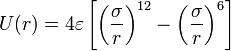 Lennard Jones potential
 - when electrostatic charges are present, we add the Coulomb force, where Q1, Q2 are the charges and ϵ0 is the permittivity of free space
- The Lennard-Jones potential is the most commonly used form, with two parameters: σ, the diameter, and ε, the well depth. It takes into account the Van der Waals forces. It represents the non-bonded forces and the total potential energy can be calculated from the sum of energy contributions between pairs of atoms.


- the bonded interactions: angles, bonds and dihedral angles have to be taken into account

Too understand a bit more, you can see the following article:
Introduction to Molecular Dynamics Simulation - Michael P. Allen
To envisage
- Molecular mutationnal assay
Already done
Here is our first movie from the modeling, showing the behavior of the protein in the dark state condition: Dark State
After having modified some parameters in the parameter files, here is our second movie, concerning the light state of the protein this time, with the FMN: Light State with FMN without water